Napa-FFT(2) implementation notes
TL;DR: program-generated Common Lisp for a memory-bound task (FFT) can reach runtime performance identical to solid C code (djbfft), and close to the state of the art (FFTW).
Discrete fourier transforms are an interesting case study in high-performance computing: they’re extremely regular recursive computations, completely free of control dependencies, and memory-bound. The recursiveness and regularity means they can be expressed or generated with relatively little code, freedom of control dependency makes them easier to benchmark, and memory-boundedness ensures that low-level instruction-selection issues can mostly be ignored. Basically, they’re perfect for specialised compilers that generate Common Lisp code. With SBCL, we have decent control over how things are laid out in memory and reasonable compilation of high-level constructs like function calls or complex float multiplication; its simple colouring register allocator and naïve code generation sometimes yield nasty assembly, but the net effect is virtually noise compared to the memory latency inherent to the algorithms.
I pushed Napa-FFT on github last week. It’s an implementation of Bailey’s 6-step
FFT [PDF] algorithm, which breaks DFTs of size n into 2 DFTs of size
  (with
appropriate rounding up/down when n isn’t a perfect square). I found the 6-step
algorithm interesting because it seems perfect to exploit caches. Reducing
computation size by a factor of ≈
(with
appropriate rounding up/down when n isn’t a perfect square). I found the 6-step
algorithm interesting because it seems perfect to exploit caches. Reducing
computation size by a factor of ≈ is huge: 1M complex doubles, which usually
overflows L2 or even L3 caches, becomes 1K, and that fits comfortably in most L1
caches. This huge reduction also means that the algorithm has a very shallow
recursion depth. For example, three recursion steps suffice to re-express a
DFT of 16 M complex doubles as a (large) number of 8-point DFT base
cases.
is huge: 1M complex doubles, which usually
overflows L2 or even L3 caches, becomes 1K, and that fits comfortably in most L1
caches. This huge reduction also means that the algorithm has a very shallow
recursion depth. For example, three recursion steps suffice to re-express a
DFT of 16 M complex doubles as a (large) number of 8-point DFT base
cases.
I completely failed to realize the latter characteristic, and I feel the approach taken in Napa-FFT is overly complex. This is where Napa-FFT2 comes in. It’s a complete rewrite of the same general idea, but explicitly structured to exploit the shallow recursion depth. This suffices to yield routines that perform comparably to djbfft on small or medium inputs, and only 25-50% slower than FFTW on large inputs.
1 Napa-FFT2
Napa-FFT2 features a small number of routine generators, each geared toward different input sizes. A first FFT generator handles small inputs and base cases for other routines; this family of routines is not expected to fare well on even medium inputs. A second generator is dedicated to slightly larger inputs and reduces medium FFTs to small ones, and a final generator builds upon the small and medium FFT generators to process even the largest inputs. Thus, there are at most two levels of recursion before specialised base cases are executed.
1.1 Radix-2 routine generator
The small FFT generator implements the same radix-2 approach as Bordeaux-FFT: tiny DFTs on indices in bit-reversed order, followed by lg n steps of contiguous additions or subtractions (butterflies) and multiplications by twiddle factors. Overall, it’s a very good algorithm: only the leaf DFTs aren’t on contiguous addresses, and the number of arithmetic operations is close to the best upper bounds known to date. The generator in Napa-FFT2 improves on Bordeaux-FFT by implementing larger base cases (up to n = 8), constant-folding most of the address computations and recognizing that no temporary vector is needed.
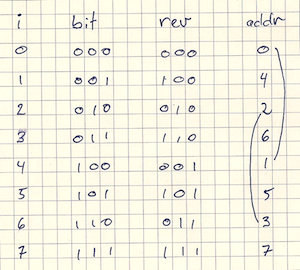
The only issue is that the access pattern needed to exploit the structure of the DFT matrix is awful on all but the smallest sizes. An L2 cache of 2 MB can only hold 128K complex doubles; for a lot of programs, temporal locality ensures most accesses hit cache even if the working set exceeds cache size. Unfortunately, the opposite happens with bit-reversed ordered accesses. The closest two indices are (e.g. they only differ in the least significant bit), the farther apart they are accessed, time-wise (see figure 1).
This explains the strong performance degradation in figure 2. The graph reports cycle counts on my 2.8 GHz X5660, which has (per core) 32 KB of L1D, 256 KB of L2, and 12 MB of L3 cache per socket. For tiny inputs, the constant overhead (function calls, the cpuid/rdtsc sequence, etc.) dominates, but, afterwards, we observe a fairly constant slope until 212, and then from 213 to 217; finally from 218 onward, performance degrades significantly. This fits well with the cache sizes. If we take into account the input, output and twiddle factor vectors, the jump from 212 to 213 overflows L2, and 217 to 218 L3.

1.2 2/4/6-step FFT algorithms
This is the effect that the 6-step algorithm attempts to alleviate. Each recursive FFT is significantly smaller: transforms of size 218, which overflows L3, are executed as transforms of size 29, which fits in L1. The total algorithmic complexity of the transform isn’t improved, but the locality of memory accesses is.
Gentleman and Sande describe how the DFT on a vector can be re-expressed as multiple DFTs on columns of row-major matrices, plus a transposition and an element-wise multiplication by a close cousin of the DFT matrix (figure 3). The transposition is nearly free of arithmetic, while the element-wise multiplication only involves streaming memory accesses, so fusing them makes a lot of sense.
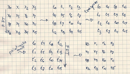
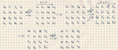
The 6-step algorithm adds two transposition steps, before and after the four steps. This way, each sub-FFT operates on adjacent addresses (figure 4), and the output is in the correct order.
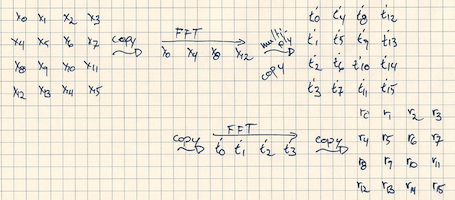
Finally, the 2-step algorithm (also found in Bailey’s paper [PDF]) is a hybrid of the 4 and 6 -step algorithms (figure 5). Rather than inserting transposition steps, columns are copied to temporary vectors before FFTing them and copying them back. Of course, the intermediate transposition and element-wise multiplication can be fused with the copy from temporary vectors.
1.3 Recursively transposing matrices
Transpositions represent a significant portion of the runtime for both 6-step algorithms. This isn’t surprising: good FFTs are memory-bound, and the only steps that aren’t cache-friendly are the three transpositions. Napa-FFT2 generates the initial and final transpositions separately from the middle 4 steps of the 6-step algorithms. This makes it easier to exploit out-of-order input or output.
It also enables us to estimate the time elapsed during each transposition step compared to the rest of the computation (for the range of sizes considered, from 26 to 225 points). Depending on the size of the input (odd or even powers of two), each transposition (initial or final) adds 5-20% of the runtime of the middle steps. With some algebra we find that, for a full DFT with in-order input and output, the three transposition steps (initial, middle and final) represent 13-40% of the total runtime!
1.3.1 Transposing square matrices
Transposition steps are faster for input sizes that are even powers of two (n = 22k). The reason is that the corresponding transposition operates on square matrices of size 2k× 2k. These are easily implemented recursively, by decomposing each matrix in four blocks until the base size is reached.
![[ | ] [ ′| ′ ]
A |B A | C
-----|----- - → -----|------
C |D B ′|D ′
| |](http://www.pvk.ca/Blog/resources/napa-fft2-implementation-notes3x.png)
As figure 6 shows, a matrix of size 2k× 2k can be transposed in-place by transposing each quadrant in-place, and swapping the top-right and bottom-left quadrants. Napa-FFT2 instead transposes the top-left and bottom-right quadrants in-place, and simultaneously transposes and swaps the two other. The in-place transpositions are simply decomposed recursively. Transpose-and-swap operations are similarly recursively decomposed into four smaller transpose-and-swaps. This recursive decomposition ensures that, for each level of the memory hierarchy (e.g. L1D cache, L2, TLB, L3), some recursion depth is well-suited to that level’s size.
The iterative base case for in-place transposition is not quite a trivial loop nest, so it’s just two nested for loops. Thankfully, it’s only used for blocks directly on the diagonal; it probably doesn’t matter much. Transpose-and-swap is simpler, and represents the vast majority of the computation. The loop nest is manually unrolled-and-jammed to improve spatial locality of the routine, and fully (or nearly) use the data brought in by each cache miss: the outer loop is partially unrolled, and the duplicated inner loops fused (everyone keeps referring to Allen and Cocke’s “A catalogue of optimizing transformations,” but I can’t find any relevant link, sorry). In figure 7, assuming that matrices A and B are in row-major order, accesses to A are naturally in streaming order; the short inner-most loop helps maximise the reuse of (non-consecutive) cache lines in B.
for i below n by 4
  for j below m
    for ii from i below i+4
      operate on A(ii, j), B(j, ii), etc.
1.3.2 Transposing rectangular matrices
Transposing general rectangular matrices is much more difficult than for square, power-of-two–sized, matrices. However, the 6-step algorithms only need to transpose matrices of size 2k× 2k+1 or 2k+1× 2k. For these shapes, it’s possible to split the input in two square block submatrices, transpose them in-place, and interleave or de-interleave the rows (figure 8).
![⌊ a′ ⌋ ⌊ ′ | ′ ⌋
[ ] | a0′ | a0 |b 0
A || a1′ || | a′ |b ′ |
------ - → ||---b2′--|| - → |⌈ 1′ | 1′ |⌉
B |⌈ b0′ |⌉ a2 |b 2
b1′ |
2](http://www.pvk.ca/Blog/resources/napa-fft2-implementation-notes4x.png)
For now, though, I found it simpler to implement that by transposing the submatrices out-of-place, moving the result to temporary storage (figure 9). The data, implicitly (de-)interleaved, is then copied back.
![[ ]
A [ | ]
------ - → A ′ |B ′
B |](http://www.pvk.ca/Blog/resources/napa-fft2-implementation-notes5x.png)
This simplistic implementation explains a lot of the slowdown on odd powers of two sizes. However, even the in-place algorithm would probably be somewhat slower than a square in-place transpose of comparable size: copying rows and tracking whether they have already been swapped into place would still use a lot of cycles.
I believe the block copies could be simplified by going through the MMU.
Matrices of 128K complex doubles or more will go through block copies (or swap) of
at least 4 KB…the usual page size on x86oids. If the vectors are correctly aligned, we
can instead remap pages in the right order. This is far from free, but it may well be
faster than actually copying the data. We’re constantly paying for address translation
but rarely do anything but mmap address space in; why not try and exploit the
hardware better?
1.4 Choosing algorithms
The medium FFT generator produces code for the 2-step algorithm, with smaller FFTs computed by specialised radix-2 code. The copy/FFT/copy loops are manually unroll-and-jammed here too.
The large FFT generator produces code for the 6-step algorithm (without the initial and final transpositions), with smaller FFTs computed either by the radix-2 or 2-step algorithms; the transposition generator is exposed separately. I assume that out-of-order output is acceptable, and only transpose the input, in place. A final transposition would be necessary to obtain in-order output.
Figure 10 lets us compare the performance of the 4 methods (radix-2, 2-step, 6-step/radix-2 and 6-step/2-step).
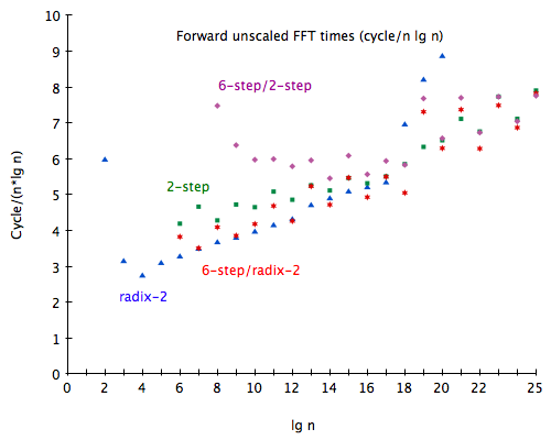
Again, radix-2 shows a severe performance degradation as soon as the working set exceeds L3 size. Both 6-step algorithms show spikes in runtimes on odd powers of two: the transposition code isn’t in-place for these vector sizes. On smaller inputs (below ≈ 210), 6-step/2-step seems dominated by constant overhead, while the spikes are on even powers of two for 6-step/radix-2. I’m not sure why this is the case for 6-step/radix-2, but the reverse for 2-step.
Table 1 shows the same data, but scaled by the lowest cycle count for each input size; I don’t have confidence intervals, but the spread was extremely low, on the order of 1%.
| lg n | Radix-2 | 2-step | 6-step/radix-2 | 6-step/2-step |
| 2 | 1.00 | |||
| 3 | 1.00 | |||
| 4 | 1.00 | |||
| 5 | 1.00 | |||
| 6 | 1.00 | 1.28 | 1.17 | |
| 7 | 1.00 | 1.34 | 1.01 | |
| 8 | 1.00 | 1.17 | 1.12 | 2.04 |
| 9 | 1.00 | 1.24 | 1.02 | 1.68 |
| 10 | 1.00 | 1.17 | 1.05 | 1.51 |
| 11 | 1.00 | 1.23 | 1.13 | 1.45 |
| 12 | 1.01 | 1.14 | 1.00 | 1.36 |
| 13 | 1.00 | 1.12 | 1.11 | 1.27 |
| 14 | 1.04 | 1.08 | 1.00 | 1.16 |
| 15 | 1.00 | 1.07 | 1.08 | 1.20 |
| 16 | 1.06 | 1.08 | 1.00 | 1.13 |
| 17 | 1.00 | 1.03 | 1.03 | 1.11 |
| 18 | 1.38 | 1.16 | 1.00 | 1.15 |
| 19 | 1.30 | 1.00 | 1.15 | 1.21 |
| 20 | 1.41 | 1.04 | 1.00 | 1.04 |
| 21 | 1.00 | 1.04 | 1.08 | |
| 22 | 1.08 | 1.00 | 1.07 | |
| 23 | 1.03 | 1.00 | 1.03 | |
| 24 | 1.04 | 1.00 | 1.03 | |
| 25 | 1.02 | 1.01 | 1.00 | |
Radix-2 provides the best performance until n = 212, at which point 6-step/radix-2 is better for even powers of two. As input size grows, the gap between radix-2 and 2-step narrows, until n = 219, at which point 2-step becomes faster than radix-2. Finally, from n = 222 onward, 6-step/radix-2 is faster than both radix-2 and 2-step.
On ridiculously large inputs (225 points or more) 6-step/2-step seems to becomes slightly faster than 6-step/radix-2, reflecting the narrowing gap between radix-2 and 2-step at sizes around 213 and greater. At first sight, it seems interesting to implement 6-step/6-step/radix-2, but this table is for out-of-order results; the 6-step algorithms depend on in-order results from the sub-FFTs, and, for those, 2-step consistently performs better.
2 Napa-FFT2, Bordeaux-FFT, djbfft and FFTW
Choosing the fastest method for each input size, from 22 to 225, yields the full implementation of Napa-FFT2. The graph in figure 11 illustrates the performance of Bordeaux-FFT, Napa-FFT2 without the final transpose for 6-step, djbfft (which lacks transforms past 213) with out-of-order output, and FFTW (the fastest of in-place and out-of-place for each size, at default planning settings). Napa-FFT2’s, or, rather, radix-2’s, performance curve is pretty much the same as djbfft’s until djbfft’s maximum size is reached. It’s interesting to note that djbfft is written in hand-tuned C, while Napa-FFT2 is machine-generated (SB)CL, without any low-level annotation except type declarations and the elimination of runtime safety checks.
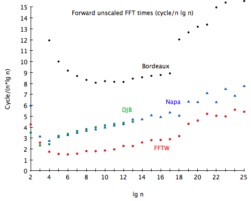
Table 2 presents the same data, scaled by the lowest cycle count. FFTW consistently has the lowest cycle counts. Napa-FFT2 and djbfft are both around twice as slow on small and medium inputs, and, on larger inputs, Napa-FFT2 becomes only 25% to 50% slower than FFTW. Bordeaux-FFT, however, is always around 3 times (or more) as slow as FFTW, and more than 50% slower than Napa-FFT2.
| lg n | Bordeaux | Napa | djb | FFTW |
| 2 | 7.26 | 1.71 | 1.00 | 1.21 |
| 3 | 7.04 | 1.35 | 1.00 | 1.11 |
| 4 | 6.83 | 1.57 | 1.39 | 1.00 |
| 5 | 6.46 | 2.00 | 2.06 | 1.00 |
| 6 | 6.10 | 2.18 | 2.25 | 1.00 |
| 7 | 5.52 | 2.22 | 2.32 | 1.00 |
| 8 | 4.60 | 2.03 | 2.11 | 1.00 |
| 9 | 4.48 | 2.11 | 2.22 | 1.00 |
| 10 | 4.41 | 2.13 | 2.24 | 1.00 |
| 11 | 4.15 | 2.11 | 2.19 | 1.00 |
| 12 | 3.57 | 1.87 | 1.93 | 1.00 |
| 13 | 3.73 | 2.08 | 1.98 | 1.00 |
| 14 | 3.29 | 1.82 | 1.00 | |
| 15 | 3.10 | 1.81 | 1.00 | |
| 16 | 3.11 | 1.74 | 1.00 | |
| 17 | 3.08 | 1.84 | 1.00 | |
| 18 | 3.78 | 1.59 | 1.00 | |
| 19 | 2.95 | 1.47 | 1.00 | |
| 20 | 2.86 | 1.37 | 1.00 | |
| 21 | 2.56 | 1.36 | 1.00 | |
| 22 | 2.97 | 1.25 | 1.00 | |
| 23 | 3.09 | 1.50 | 1.00 | |
| 24 | 2.83 | 1.23 | 1.00 | |
| 25 | 2.87 | 1.43 | 1.00 | |
3 What’s next?
The prototype is already pretty good, and definitely warrants more hacking. There are a few obvious things on my list:
- Most of the improvements in the radix-2 generator (larger base cases and making the temporary vector useless) can be ported to Bordeaux-FFT;
- Both the small FFT generator and Bordeaux-FFT could benefit from a split-radix (radix-2/4 instead radix-2) rewrite;
- Scaling (during copy or transpose) is already coded, it must simply be enabled;
- Inverse transforms would be useful;
- In-place rectangular transpositions would probably help reduce the performance gap between odd and even powers of two for the 6-step algorithms;
- Processing real input specially can lead to hugely faster code with little work;
- Generalizing the transposition code to handle arbitrary (power-of-two–sized) matrices would enable easy multidimensional FFTs;
- Finally, I must write a library instead of writing base cases, constant-folding address computations or unrolling (and jamming) loops by hand. It would pretty much be a compiler geared toward large recursively-generated, but repetitive and simple, array-manipulation code.
It’s pretty clear that SBCL’s native support on x86-64 for SSE2 complex float arithmetic pays off. I expect other tasks would similarly benefit from hand-written assembly routines for a few domain-specific operations. SBCL’s architecture makes that very easy. It’s when we want to rewrite patterns across function calls that Python gets in the way…and that’s exactly what code generators should be concerned with getting right.
In the end, I think the most interesting result is that the runtime performance of (SB)CL can definitely be competitive with C for memory-bound tasks like FFT. Common Lisp compilers generally suffer from simplistic, 70’s-style, low-level code generation facilities; luckily, when tackling memory-bound tasks, getting the algorithms and data layouts right to reduce the operation count and exploit hierarchical memory matters a lot more. The advantage of CL is that, unlike C, it’s easy to generate and compile, even at runtime. CL is also easier to debug, since we can enable or disable runtime checks with a single declaration.
If the trend of memory bandwidth (and latency) improving much more slowly than computing power persists, while we keep processing larger data sets, the suitability of Common Lisp to the generation of high-performance code is an asset that will prove itself more and more useful in the near future.
I’m also pleasantly surprised by the performance of Napa-FFT2, regardless of the target language. I’ll probably try and re-implement it in runtime-specialised C (VLBDB, another side-project of mine). This would hopefully help close the gap with FFTW even further, and make it easier to try and exploit MMU tricks.
