I previously noted how preemption makes lock-free programming harder in userspace than in the kernel. I now believe that preemption ought to be treated as a sunk cost, like garbage collection: we’re already paying for it, so we might as well use it. Interrupt processing (returning from an interrupt handler, actually) is fully serialising on x86, and on other platforms, no doubt: any userspace instruction either fully executes before the interrupt, or is (re-)executed from scratch some time after the return back to userspace. That’s something we can abuse to guarantee ordering between memory accesses, without explicit barriers.
This abuse of interrupts is complementary to Bounded TSO. Bounded TSO measures the hardware limit on the number of store instructions that may concurrently be in-flight (and combines that with the knowledge that instructions are retired in order) to guarantee liveness without explicit barriers, with no overhead, and usually marginal latency. However, without worst-case execution time information, it’s hard to map instruction counts to real time. Tracking interrupts lets us determine when enough real time has elapsed that earlier writes have definitely retired, albeit after a more conservative delay than Bounded TSO’s typical case.
I reached this position after working on two lock-free synchronisation primitives—event counts, and asymmetric flag flips as used in hazard pointers and epoch reclamation—that are similar in that a slow path waits for a sign of life from a fast path, but differ in the way they handle “stuck” fast paths. I’ll cover the event count and flag flip implementations that I came to on Linux/x86[-64], which both rely on interrupts for ordering. Hopefully that will convince you too that preemption is a useful source of pre-paid barriers for lock-free code in userspace.
I’m writing this for readers who are already familiar with
lock-free programming,
safe memory reclamation techniques in particular, and have some
experience reasoning with formal memory models.
For more references, Samy’s overview in the ACM Queue is a good resource.
I already committed the code for
event counts in Concurrency Kit,
and for interrupt-based reverse barriers in my barrierd project.
Event counts with x86-TSO and futexes
An event count
is essentially a version counter that lets threads wait
until the current version differs from an arbitrary prior version. A
trivial “wait” implementation could spin on the version counter.
However, the value of event counts is that they let lock-free code
integrate with OS-level blocking: waiters can grab the event count’s
current version v0, do what they want with the versioned data, and
wait for new data by sleeping rather than burning cycles until the
event count’s version differs from v0. The event count is a common
synchronisation primitive that is often reinvented and goes by many
names (e.g.,
blockpoints);
what matters is that writers can update the version counter, and
waiters can read the version, run arbitrary code, then efficiently
wait while the version counter is still equal to that previous
version.
The explicit version counter solves the lost wake-up issue associated with misused condition variables, as in the pseudocode below.
bad condition waiter:

while True:
    atomically read data
    if need to wait:
        WaitOnConditionVariable(cv)
    else:
        break
In order to work correctly, condition variables require waiters to acquire a mutex that protects both data and the condition variable, before checking that the wait condition still holds and then waiting on the condition variable.
good condition waiter:

while True:
    with(mutex):
        read data
        if need to wait:
	        WaitOnConditionVariable(cv, mutex)
	    else:
	        break Waiters must prevent writers from making changes to the data, otherwise the data change (and associated condition variable wake-up) could occur between checking the wait condition, and starting to wait on the condition variable.  The waiter would then have missed a wake-up and could end up sleeping forever, waiting for something that has already happened.

good condition waker:

with(mutex):
    update data
    SignalConditionVariable(cv)
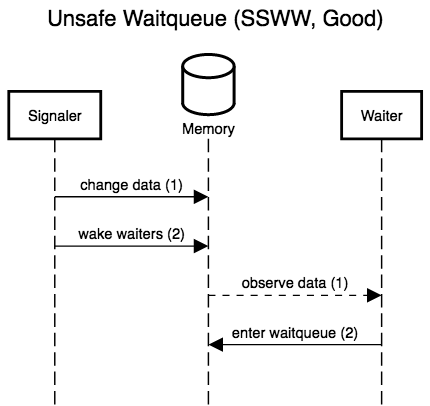
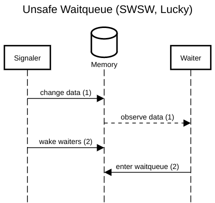
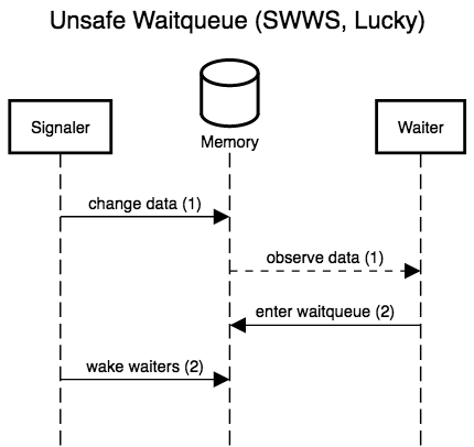
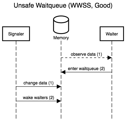
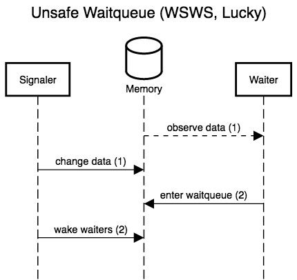
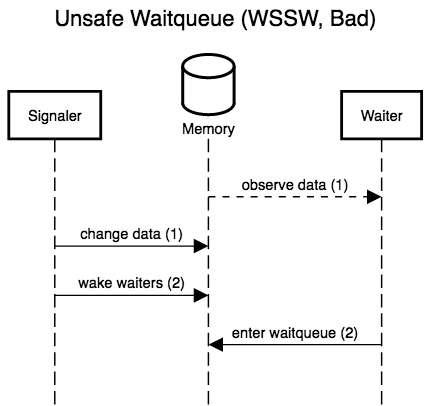
The six diagrams below show the possible interleavings between the
signaler (writer) making changes to the data and waking waiters, and
a waiter observing the data and entering the queue to wait for
changes. The two left-most diagrams don’t interleave anything; these
are the only scenarios allowed by correct locking. The remaining four
actually interleave the waiter and signaler, and show that, while
three are accidentally correct (lucky), there is one case, WSSW,
where the waiter misses its wake-up.
If any waiter can prevent writers from making progress, we don’t have a lock-free protocol. Event counts let waiters detect when they would have been woken up (the event count’s version counter has changed), and thus patch up this window where waiters can miss wake-ups for data changes they have yet to observe. Crucially, waiters detect lost wake-ups, rather than preventing them by locking writers out. Event counts thus preserve lock-freedom (and even wait-freedom!).
We could, for example, use an event count in a lock-free ring buffer: rather than making consumers spin on the write pointer, the write pointer could be encoded in an event count, and consumers would then efficiently block on that, without burning CPU cycles to wait for new messages.
The challenging part about implementing event counts isn’t making sure
to wake up sleepers, but to only do so when there are sleepers to
wake. For some use cases, we don’t need to do any active wake-up,
because exponential backoff is good enough: if version updates
signal the arrival of a response in a request/response communication
pattern, exponential backoff, e.g., with a 1.1x backoff factor,
could bound the increase in response latency caused by the blind sleep
during backoff, e.g., to 10%.
Unfortunately, that’s not always applicable. In general, we can’t assume that signals corresponds to responses for prior requests, and we must support the case where progress is usually fast enough that waiters only spin for a short while before grabbing more work. The latter expectation means we can’t “just” unconditionally execute a syscall to wake up sleepers whenever we increment the version counter: that would be too slow. This problem isn’t new, and has a solution similar to the one deployed in adaptive spin locks.
The solution pattern for adaptive locks relies on tight integration with an OS primitive, e.g., futexes. The control word, the machine word on which waiters spin, encodes its usual data (in our case, a version counter), as well as a new flag to denote that there are sleepers waiting to be woken up with an OS syscall. Every write to the control word uses atomic read-modify-write instructions, and before sleeping, waiters ensure the “sleepers are present” flag is set, then make a syscall to sleep only if the control word is still what they expect, with the sleepers flag set.
OpenBSD’s compatibility shim for Linux’s futexes is about as simple an implementation of the futex calls as it gets. The OS code for futex wake and wait is identical to what userspace would do with mutexes and condition variables (waitqueues). Waiters lock out wakers for the futex word or a coarser superset, check that the futex word’s value is as expected, and enters the futex’s waitqueue. Wakers acquire the futex word for writes, and wake up the waitqueue. The difference is that all of this happens in the kernel, which, unlike userspace, can force the scheduler to be helpful. Futex code can run in the kernel because, unlike arbitrary mutex/condition variable pairs, the protected data is always a single machine integer, and the wait condition an equality test. This setup is simple enough to fully implement in the kernel, yet general enough to be useful.
OS-assisted conditional blocking is straightforward enough to adapt to event counts. The control word is the event count’s version counter, with one bit stolen for the “sleepers are present” flag (sleepers flag).
Incrementing the version counter can use a regular atomic increment; we only need to make sure we can tell whether the sleepers flag might have been set before the increment. If the sleepers flag was set, we clear it (with an atomic bit reset), and wake up any OS thread blocked on the control word.
increment event count:

old <- fetch_and_add(event_count.counter, 2)  # flag is in the low bit
if (old & 1):
    atomic_and(event_count.counter, -2)
    signal waiters on event_count.counter
Waiters can spin for a while, waiting for the version counter to change. At some point, a waiter determines that it’s time to stop wasting CPU time. The waiter then sets the sleepers flag with a compare-and-swap: the CAS (compare-and-swap) can only fail because the counter’s value has changed or because the flag is already set. In the former failure case, it’s finally time to stop waiting. In the latter failure care, or if the CAS succeeded, the flag is now set. The waiter can then make a syscall to block on the control word, but only if the control word still has the sleepers flag set and contains the same expected (old) version counter.
wait until event count differs from prev:

repeat k times:
    if (event_count.counter / 2) != prev:  # flag is in low bit.
        return
compare_and_swap(event_count.counter, prev * 2, prev * 2 + 1)
if cas_failed and cas_old_value != (prev * 2 + 1):
    return
repeat k times:
    if (event_count.counter / 2) != prev:
        return
sleep_if(event_count.center == prev * 2 + 1)
This scheme works, and offers decent performance. In fact, it’s good
enough for Facebook’s Folly.
I certainly don’t see how we can improve on that if there are
concurrent writers (incrementing threads).
However, if we go back to the ring buffer example, there is often only
one writer per ring. Enqueueing an item in a
single-producer ring buffer incurs no atomic, only a release store:
the write pointer increment only has to be visible after the data
write, which is always the case under the TSO memory model (including
x86). Replacing the write pointer in a single-producer ring buffer
with an event count where each increment incurs an atomic operation is
far from a no-brainer. Can we do better, when there is only one
incrementer?
On x86 (or any of the zero other architectures with non-atomic read-modify-write instructions and TSO), we can… but we must accept some weirdness.
The operation that must really be fast is incrementing the event counter, especially when the sleepers flag is not set. Setting the sleepers flag on the other hand, may be slower and use atomic instructions, since it only happens when the executing thread is waiting for fresh data.
I suggest that we perform the former, the increment on the fast path,
with a non-atomic read-modify-write instruction, either inc mem or
xadd mem, reg. If the sleepers flag is in the sign bit, we can
detect it (modulo a false positive on wrap-around) in the condition
codes computed by inc; otherwise, we must use xadd (fetch-and-add)
and look at the flag bit in the fetched value.
The usual ordering-based arguments are no help in this kind of
asymmetric synchronisation pattern. Instead, we must go directly to
the x86-TSO
memory model. All atomic (LOCK prefixed) instructions conceptually
flush the executing core’s store buffer, grab an exclusive lock on
memory, and perform the read-modify-write operation with that lock
held. Thus, manipulating the sleepers flag can’t lose updates that
are already visible in memory, or on their way from the store buffer.
The RMW increment will also always see the latest version update
(either in global memory, or in the only incrementer’s store buffer),
so won’t lose version updates either. Finally, scheduling and thread
migration must always guarantee that the incrementer thread sees its
own writes, so that won’t lose version updates.
increment event count without atomics in the common case:

old <- non_atomic_fetch_and_add(event_count.counter, 2)
if (old & 1):
    atomic_and(event_count.counter, -2)
    signal waiters on event_count.counter
The only thing that might be silently overwritten is the sleepers flag: a waiter might set that flag in memory just after the increment’s load from memory, or while the increment reads a value with the flag unset from the local store buffer. The question is then how long waiters must spin before either observing an increment, or knowing that the flag flip will be observed by the next increment. That question can’t be answered with the memory model, and worst-case execution time bounds are a joke on contemporary x86.
I found an answer by remembering that IRET, the instruction used to
return from interrupt handlers, is a full barrier.1
We also know that interrupts happen at frequent and regular intervals,
if only for the preemption timer (every 4-10ms on stock Linux/x86oid).
Regardless of the bound on store visibility, a waiter can flip the sleepers-are-present flag, spin on the control word for a while, and then start sleeping for short amounts of time (e.g., a millisecond or two at first, then 10 ms, etc.): the spin time is long enough in the vast majority of cases, but could still, very rarely, be too short.
At some point, we’d like to know for sure that, since we have yet to observe a silent overwrite of the sleepers flag or any activity on the counter, the flag will always be observed and it is now safe to sleep forever. Again, I don’t think x86 offers any strict bound on this sort of thing. However, one second seems reasonable. Even if a core could stall for that long, interrupts fire on every core several times a second, and returning from interrupt handlers acts as a full barrier. No write can remain in the store buffer across interrupts, interrupts that occur at least once per second. It seems safe to assume that, once no activity has been observed on the event count for one second, the sleepers flag will be visible to the next increment.
That assumption is only safe if interrupts do fire at regular intervals. Some latency sensitive systems dedicate cores to specific userspace threads, and move all interrupt processing and preemption away from those cores. A correctly isolated core running Linux in tickless mode, with a single runnable process, might not process interrupts frequently enough. However, this kind of configuration does not happen by accident. I expect that even a half-second stall in such a system would be treated as a system error, and hopefully trigger a watchdog. When we can’t count on interrupts to get us barriers for free, we can instead rely on practical performance requirements to enforce a hard bound on execution time.
Either way, waiters set the sleepers flag, but can’t rely on it being observed until, very conservatively, one second later. Until that time has passed, waiters spin on the control word, then block for short, but growing, amounts of time. Finally, if the control word (event count version and sleepers flag) has not changed in one second, we assume the incrementer has no write in flight, and will observe the sleepers flag; it is safe to block on the control word forever.
wait until event count differs from prev:

repeat k times:
    if (event_count.counter / 2) != prev:
        return
compare_and_swap(event_count.counter, 2 * prev, 2 * prev + 1)
if cas_failed and cas_old_value != 2 * prev + 1:
    return
repeat k times:
    if event_count.counter != 2 * prev + 1:
        return
repeat for 1 second:
    sleep_if_until(event_count.center == 2 * prev + 1,
                   $exponential_backoff)
    if event_count.counter != 2 * prev + 1:
        return
sleep_if(event_count.center == prev * 2 + 1)
That’s the solution I implemented in this pull request for
SPMC and MPMC event counts in concurrency kit.
The MP (multiple producer) implementation is the regular adaptive
logic, and matches Folly’s strategy. It needs about 30 cycles for an
uncontended increment with no waiter, and waking up sleepers adds
another 700 cycles on my E5-46xx (Linux 4.16). The single producer
implementation is identical for the slow path, but only takes ~8
cycles per increment with no waiter, and, eschewing atomic
instruction, does not flush the pipeline (i.e., the out-of-order
execution engine is free to maximise throughput). The additional
overhead for an increment without waiter, compared to a regular ring
buffer pointer update, is 3-4 cycles for a single predictable conditional branch or fused
test and branch, and the RMW’s load instead of a regular
add/store. That’s closer to zero overhead, which makes it much easier
for coders to offer OS-assisted blocking in their lock-free
algorithms, without agonising over the penalty when no one needs to
block.
Asymmetric flag flip with interrupts on Linux
Hazard pointers and epoch reclamation. Two different memory reclamation technique, in which the fundamental complexity stems from nearly identical synchronisation requirements: rarely, a cold code path (which is allowed to be very slow) writes to memory, and must know when another, much hotter, code path is guaranteed to observe the slow path’s last write.
For hazard pointers, the cold code path waits until, having overwritten an object’s last persistent reference in memory, it is safe to destroy the pointee. The hot path is the reader:
1. read pointer value *(T **)x.
2. write pointer value to hazard pointer table
3. check that pointer value *(T **)x has not changed
Similarly, for epoch reclamation, a read-side section will grab the current epoch value, mark itself as reading in that epoch, then confirm that the epoch hasn’t become stale.
1. $epoch <- current epoch
2. publish self as entering a read-side section under $epoch
3. check that $epoch is still current, otherwise retry
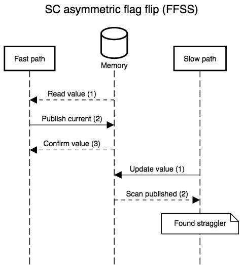
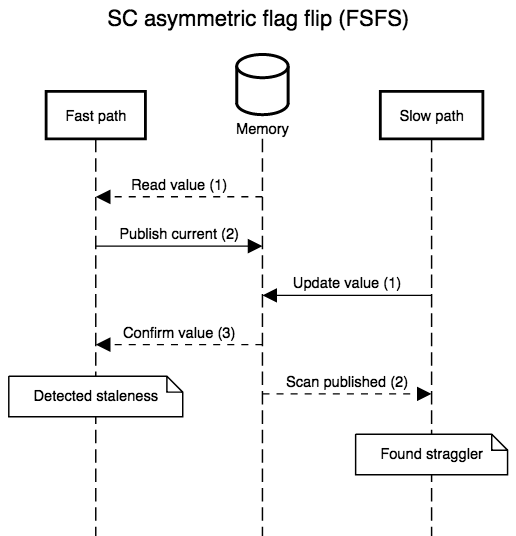
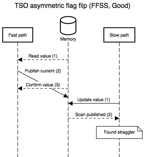
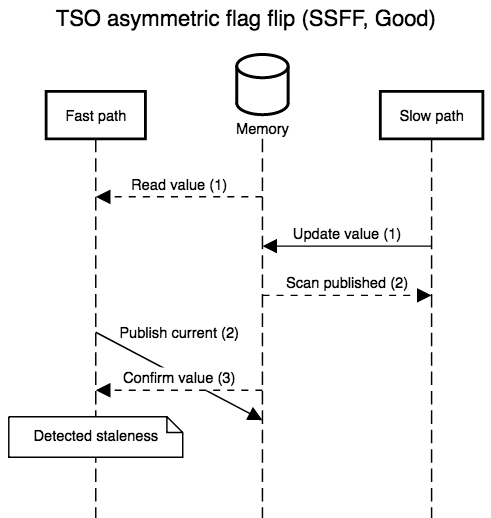
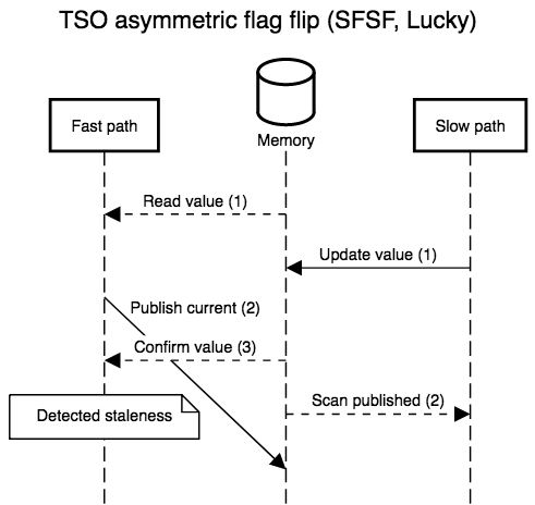
Under a sequentially consistent (SC) memory model, the two sequences are valid with regular (atomic) loads and stores. The slow path can always make its write, then scan every other thread’s single-writer data to see if any thread has published something that proves it executed step 2 before the slow path’s store (i.e., by publishing the old pointer or epoch value).
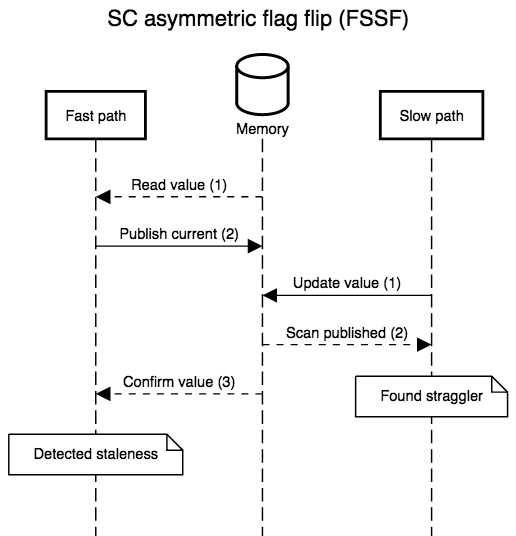
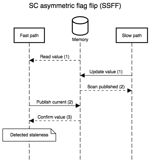
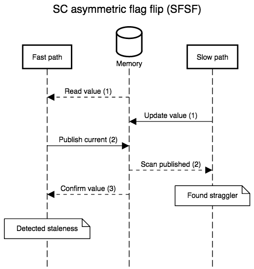
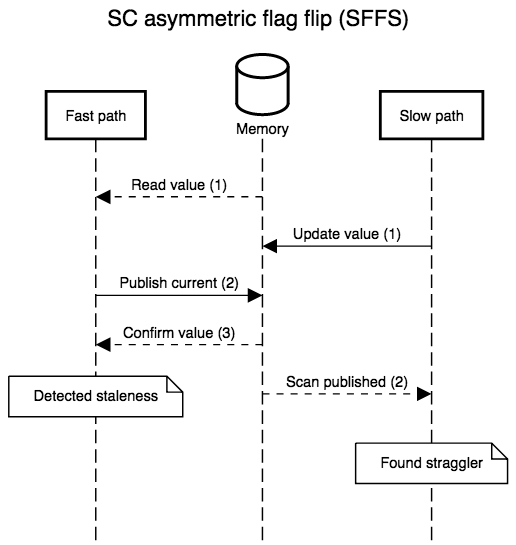
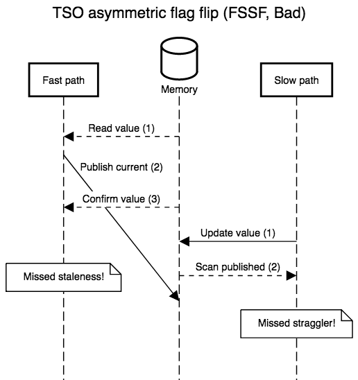
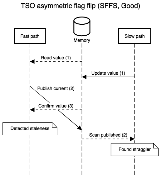
The diagrams below show all possible interleavings. In all cases, once there is no evidence that a thread has failed to observe the slow path’s new write, we can correctly assume that all threads will observe the write. I simplified the diagrams by not interleaving the first read in step 1: its role is to provide a guess for the value that will be re-read in step 3, so, at least with respect to correctness, that initial read might as well be generating random values. I also kept the second “scan” step in the slow path abstract. In practice, it’s a non-snapshot read of all the epoch or hazard pointer tables for threads that execute the fast path: the slow path can assume an epoch or pointer will not be resurrected once the epoch or pointer is absent from the scan.
No one implements SC in hardware. X86 and SPARC offer the strongest
practical memory model, Total Store Ordering, and that’s
still not enough to correctly execute the read-side critical sections
above without special annotations. Under TSO, reads (e.g., step 3)
are allowed to execute before writes (e.g., step 2).
X86-TSO models
that as a buffer in which stores may be delayed, and that’s what the
scenarios below show, with steps 2 and 3 of the fast path reversed
(the slow path can always be instrumented to recover sequential order,
it’s meant to be slow). The TSO interleavings only differ from the SC
ones when the fast path’s steps 2 and 3 are separated by something on
slow path’s: when the two steps are adjacent, their order relative to
the slow path’s steps is unaffected by TSO’s delayed stores. TSO is so
strong that we only have to fix one case, FSSF, where the slow path
executes in the middle of the fast path, with the reversal of store
and load order allowed by TSO.
Simple implementations plug this hole with a store-load barrier between the second and third steps, or implement the store with an atomic read-modify-write instruction that doubles as a barrier. Both modifications are safe and recover SC semantics, but incur a non-negligible overhead (the barrier forces the out of order execution engine to flush before accepting more work) which is only necessary a minority of the time.
The pattern here is similar to the event count, where the slow path signals the fast path that the latter should do something different. However, where the slow path for event counts wants to wait forever if the fast path never makes progress, hazard pointer and epoch reclamation must detect that case and ignore sleeping threads (that are not in the middle of a read-side SMR critical section).
In this kind of asymmetric synchronisation pattern, we wish to move as
much of the overhead to the slow (cold) path. Linux 4.3 gained the
membarrier
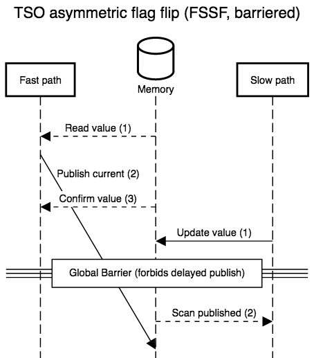
syscall for exactly this use case. The slow path can execute its
write(s) before making a membarrier syscall. Once the syscall
returns, any fast path write that has yet to be visible (hasn’t
retired yet), along with every subsequent instruction in program
order, started in a state where the slow path’s writes were visible.
As the next diagram shows, this global barrier lets us rule out the
one anomalous execution possible under TSO, without adding any special
barrier to the fast path.
The problem with membarrier is that it comes in two flavours: slow,
or not scalable. The initial, unexpedited, version waits for kernel
RCU to run its callback, which, on my machine, takes anywhere between
25 and 50 milliseconds. The reason it’s so slow is that the
condition for an RCU grace period to elapse are more demanding than
a global barrier, and may even require multiple such
barriers. For example, if we used the same scheme to nest epoch
reclamation ten deep, the outermost reclaimer would be 1024 times
slower than the innermost one. In reaction to this slowness,
potential users of membarrier went back to triggering
IPIs, e.g.,
by mprotecting a dummy page.
mprotect isn’t guaranteed to act as a barrier, and does not do so on
AArch64, so Linux 4.16 added an “expedited” mode to membarrier. In
that expedited mode, each membarrier syscall sends an IPI to every
other core… when I look at machines with hundreds of cores, \(n -
1\) IPI per core, a couple times per second on every \(n\) core,
start to sound like a bad idea.
Let’s go back to the observation we made for event count: any interrupt acts as a barrier for us, in that any instruction that retires after the interrupt must observe writes made before the interrupt. Once the hazard pointer slow path has overwritten a pointer, or the epoch slow path advanced the current epoch, we can simply look at the current time, and wait until an interrupt has been handled at a later time on all cores. The slow path can then scan all the fast path state for evidence that they are still using the overwritten pointer or the previous epoch: any fast path that has not published that fact before the interrupt will eventually execute the second and third steps after the interrupt, and that last step will notice the slow path’s update.
There’s a lot of information in /proc that lets us conservatively
determine when a new interrupt has been handled on every core.
However, it’s either too granular (/proc/stat) or
extremely slow to generate (/proc/schedstat). More importantly,
even with ftrace, we can’t easily ask to be woken up when something
interesting happens, and are forced to poll files for updates
(never mind the weirdly hard to productionalise kernel interface).
What we need is a way to read, for each core, the last time it was
definitely processing an interrupt. Ideally, we could also block and
let the OS wake up our waiter on changes to the oldest “last
interrupt” timestamp, across all cores. On x86, that’s enough to get
us the asymmetric barriers we need for hazard pointers and epoch
reclamation, even if only IRET is serialising, and not
interrupt handler entry. Once a core’s update to its “last interrupt”
timestamp is visible, any write prior to the update, and thus any
write prior to the interrupt is also globally visible: we can only
observe the timestamp update from a different core than the updater,
in which case TSO saves us, or after the handler has returned with a
serialising IRET.
We can bundle all that logic in a short eBPF program.2 The program has a map of thread-local arrays (of 1 CLOCK_MONOTONIC timestamp each), a map of perf event queues (one per CPU), and an array of 1 “watermark” timestamp. Whenever the program runs, it gets the current time. That time will go in the thread-local array of interrupt timestamps. Before storing a new value in that array, the program first reads the previous interrupt time: if that time is less than or equal to the watermark, we should wake up userspace by enqueueing in event in perf. The enqueueing is conditional because perf has more overhead than a thread-local array, and because we want to minimise spurious wake-ups. A high signal-to-noise ratio lets userspace set up the read end of the perf queue to wake up on every event and thus minimise update latency.
We now need a single global daemon
to attach the eBPF program to an arbitrary set of software tracepoints
triggered by interrupts (or PMU events that trigger interrupts), to
hook the perf fds to epoll, and to re-read the map of interrupt
timestamps whenever epoll detects a new perf event. That’s what the
rest of the code handles: setting up tracepoints, attaching the eBPF
program, convincing perf to wake us up, and hooking it all up to
epoll. On my fully loaded 24-core E5-46xx running Linux 4.18 with
security patches, the daemon uses ~1-2% (much less on 4.16) of
a core to read the map of timestamps every time it’s woken up every ~4
milliseconds. perf shows the non-JITted eBPF program itself uses
~0.1-0.2% of every core.
Amusingly enough, while eBPF offers maps that are safe for concurrent
access in eBPF programs, the same maps come with no guarantee when
accessed from userspace, via the syscall interface. However, the
implementation uses a hand-rolled long-by-long copy loop, and, on
x86-64, our data all fit in longs. I’ll hope that the kernel’s
compilation flags (e.g., -ffree-standing) suffice to prevent GCC
from recognising memcpy or memmove, and that we thus get atomic
store and loads on x86-64. Given the quality of eBPF documentation,
I’ll bet that this implementation accident is actually part of
the API. Every BPF map is single writer (either per-CPU in the
kernel, or single-threaded in userspace), so this should work.
Once the barrierd daemon is running, any program can mmap its data
file to find out the last time we definitely know each core had
interrupted userspace, without making any further syscall or incurring
any IPI. We can also use regular synchronisation to let the daemon
wake up threads waiting for interrupts as soon as the oldest interrupt
timestamp is updated. Applications don’t even need to call
clock_gettime to get the current time: the daemon also works in
terms of a virtual time that it updates in the mmaped data file.
The barrierd data file also includes an array of per-CPU structs
with each core’s timestamps (both from CLOCK_MONOTONIC and in virtual
time). A client that knows it will only execute on a subset of CPUs,
e.g., cores 2-6, can compute its own “last interrupt” timestamp by
only looking at entries 2 to 6 in the array. The daemon even wakes up
any futex waiter on the per-CPU values whenever they change. The
convenience interface is pessimistic, and assumes that client code
might run on every configured core. However, anyone can mmap the
same file and implement tighter logic.
Again, there’s a snag with tickless kernels. In the default
configuration already, a fully idle core might not process timer
interrupts. The barrierd daemon detects when a core is falling
behind, and starts looking for changes to /proc/stat. This backup
path is slower and coarser grained, but always works with idle cores.
More generally, the daemon might be running on a system with dedicated
cores. I thought about causing interrupts by re-affining RT threads,
but that seems counterproductive. Instead, I think the right approach
is for users of barrierd to treat dedicated cores specially.
Dedicated threads can’t (shouldn’t) be interrupted, so they can
regularly increment a watchdog counter with a serialising instruction.
Waiters will quickly observe a change in the counters for dedicated
threads, and may use barrierd to wait for barriers on preemptively
shared cores. Maybe dedicated threads should be able to
hook into barrierd and check-in from time to time. That would break
the isolation between users of barrierd, but threads on dedicated
cores are already in a privileged position.
I quickly compared the barrier latency on an unloaded 4-way E5-46xx
running Linux 4.16, with a sample size of 20000 observations per
method (I had to remove one outlier at 300ms). The synchronous
methods mprotect (which abuses mprotect to send IPIs by removing
and restoring permissions on a dummy page), or explicit IPI via
expedited membarrier, are much faster than the other (unexpedited
membarrier with kernel RCU, or barrierd that counts interrupts).
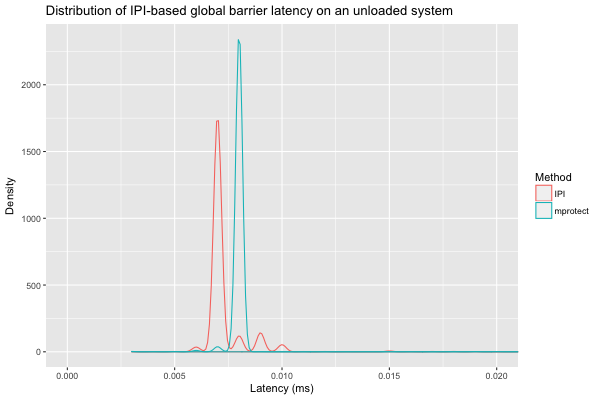
We can zoom in on the IPI-based methods, and see that an expedited
membarrier (IPI) is usually slightly faster than mprotect;
IPI via expedited membarrier hits a worst-case of 0.041 ms, versus
0.046 for mprotect.
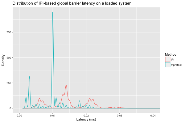
The performance of IPI-based barriers should be roughly independent of
system load. However, we did observe a slowdown for expedited
membarrier (between \(68.4-73.0\%\) of the time,
\(p < 10\sp{-12}\) according to a binomial test3) on the same
4-way system, when all CPUs were running CPU-intensive code at low
priority. In this second experiment, we have a sample size of one
million observations for each method, and the worst case for IPI via
expedited membarrier was 0.076 ms (0.041 ms on an unloaded system),
compared to a more stable 0.047 ms for mprotect.
Now for non-IPI methods: they should be slower than methods that trigger synchronous IPIs, but hopefully have lower overhead and scale better, while offering usable latencies.
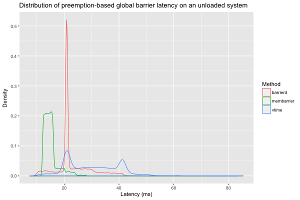
On an unloaded system, the interrupts that drive barrierd are less
frequent, sometimes outright absent, so unexpedited membarrier
achieves faster response times. We can even observe barrierd’s
fallback logic, which scans /proc/stat for evidence of idle CPUs
after 10 ms of inaction: that’s the spike at 20ms. The values for
vtime show the additional slowdown we can expect if we wait on
barrierd’s virtual time, rather than directly reading
CLOCK_MONOTONIC. Overall, the worst case latencies for barrierd
(53.7 ms) and membarrier (39.9 ms) aren’t that different, but I
should add another fallback mechanism based on membarrier to improve
barrierd’s performance on lightly loaded machines.
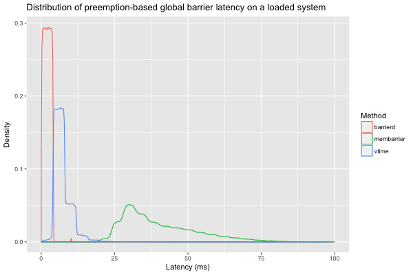
When the same 4-way, 24-core, system is under load, interrupts are
fired much more frequently and reliably, so barrierd shines, but
everything has a longer tail, simply because of preemption of the
benchmark process. Out of the one million observations we have for
each of unexpedited membarrier, barrierd, and barrierd with
virtual time on this loaded system, I eliminated 54 values over
100 ms (18 for membarrier, 29 for barrierd, and 7 for virtual
time). The rest is shown below. barrierd is consistently much
faster than membarrier, with a geometric mean speedup of 23.8x. In
fact, not only can we expect barrierd to finish before an
unexpedited membarrier \(99.99\%\) of the time
(\(p<10\sp{-12}\) according to a binomial test), but we can even expect barrierd to be 10 times as
fast \(98.3-98.5\%\) of the time (\(p<10\sp{-12}\)). The gap is
so wide that even the opportunistic virtual-time approach is faster
than membarrier (geometric mean of 5.6x), but this time with a mere
three 9s (as fast as membarrier \(99.91-99.96\%\) of the time,
\(p<10\sp{-12}\)).
With barrierd, we get implicit
barriers with worse overhead than unexpedited membarrier (which is
essentially free since it piggybacks on kernel RCU, another sunk
cost), but 1/10th the latency (0-4 ms instead of 25-50 ms). In
addition, interrupt tracking is per-CPU, not per-thread, so it only
has to happen in a global single-threaded daemon; the rest of
userspace can obtain the information it needs without causing
additional system overhead. More importantly, threads don’t have to
block if they use barrierd to wait for a system-wide barrier. That’s
useful when, e.g., a thread pool worker is waiting for a reverse
barrier before sleeping on a futex. When that worker blocks in
membarrier for 25ms or 50ms, there’s a potential hiccup where a work
unit could sit in the worker’s queue for that amount of time before it
gets processed. With barrierd (or the event count described earlier), the worker can spin and wait for work units to
show up until enough time has passed to sleep on the futex.
While I believe that information about interrupt times should be made
available without tracepoint hacks, I don’t know if a syscall like
membarrier is really preferable to a shared daemon like barrierd.
The one salient downside is that barrierd slows down when some CPUs
are idle; that’s something we can fix by including a membarrier
fallback, or by sacrificing power consumption and forcing kernel
ticks, even for idle cores.
Preemption can be an asset
When we write lock-free code in userspace, we always have preemption in mind. In fact, the primary reason for lock-free code in userspace is to ensure consistent latency despite potentially adversarial scheduling. We spend so much effort to make our algorithms work despite interrupts and scheduling that we can fail to see how interrupts can help us. Obviously, there’s a cost to making our code preemption-safe, but preemption isn’t an option. Much like garbage collection in managed language, preemption is a feature we can’t turn off. Unlike GC, it’s not obvious how to make use of preemption in lock-free code, but this post shows it’s not impossible.
We can use preemption to get asymmetric barriers, nearly for free,
with a daemon like barrierd. I see a duality between
preemption-driven barriers and techniques like Bounded TSO:
the former are relatively slow, but offer hard bounds, while the
latter guarantee liveness, usually with negligible latency, but
without any time bound.
I used preemption to make single-writer event counts faster
(comparable to a regular non-atomic counter), and to provide a
lower-latency alternative to membarrier’s asymmetric barrier.
In a similar vein,
SPeCK
uses time bounds to ensure scalability, at the expense of a bit of
latency, by enforcing periodic TLB reloads instead of relying on
synchronous shootdowns. What else can we do with interrupts, timer or
otherwise?
Thank you Samy, Gabe, and Hanes for discussions on an earlier draft. Thank you Ruchir for improving this final version.
P.S. event count without non-atomic RMW?
The single-producer event count specialisation relies on non-atomic read-modify-write instructions, which are hard to find outside x86. I think the flag flip pattern in epoch and hazard pointer reclamation shows that’s not the only option.
We need two control words, one for the version counter, and another for the sleepers flag. The version counter is only written by the incrementer, with regular non-atomic instructions, while the flag word is written to by multiple producers, always with atomic instructions.
The challenge is that OS blocking primitives like futex only let us
conditionalise the sleep on a single word. We could try to pack a
pair of 16-bit shorts in a 32-bit int, but that doesn’t give us a
lot of room to avoid wrap-around. Otherwise, we can guarantee that
the sleepers flag is only cleared immediately before incrementing the
version counter. That suffices to let sleepers only conditionalise on
the version counter… but we still need to trigger a wake-up if the
sleepers flag was flipped between the last clearing and the increment.
On the increment side, the logic looks like
must_wake = false
if sleepers flag is set:
    must_wake = true
    clear sleepers flag
increment version
if must_wake or sleepers flag is set:
    wake up waiters
and, on the waiter side, we find
if version has changed
    return
set sleepers flag
sleep if version has not changed
The separate “sleepers flag” word doubles the space usage, compared to the single flag bit in the x86 single-producer version. Composite OS uses that two-word solution in blockpoints, and the advantages seem to be simplicity and additional flexibility in data layout. I don’t know that we can implement this scheme more efficiently in the single producer case, under other memory models than TSO. If this two-word solution is only useful for non-x86 TSO, that’s essentially SPARC, and I’m not sure that platform still warrants the maintenance burden.
But, we’ll see, maybe we can make the above work on AArch64 or POWER.
-
I actually prefer another, more intuitive, explanation that isn’t backed by official documentation.The store buffer in x86-TSO doesn’t actually exist in silicon: it represents the instructions waiting to be retired in the out-of-order execution engine. Precise interrupts seem to imply that even entering the interrupt handler flushes the OOE engine’s state, and thus acts as a full barrier that flushes the conceptual store buffer. ↩
-
I used raw eBPF instead of the C frontend because that frontend relies on a ridiculous amount of runtime code that parses an ELF file when loading the eBPF snippet to know what eBPF maps to setup and where to backpatch their
fdnumber. I also find there’s little advantage to the C frontend for the scale of eBPF programs (at most 4096 instructions, usually much fewer). I did useclangto generate a starting point, but it’s not that hard to tighten 30 instructions in ways that a compiler can’t without knowing what part of the program’s semantics is essential. Thebpfsyscall can also populate a string buffer with additional information when loading a program. That’s helpful to know that something was assembled wrong, or to understand why the verifier is rejecting your program. ↩ -
I computed these extreme confidence intervals with my old code to test statistical SLOs. ↩
