This post describes how graph and automata theory can help compile a regular expression like “ab(cd|e)*fg” into the following asymptotically (linear-time) and practically (around 8 cycles/character on my E5-4617) efficient machine code. The technique is easily amenable to SSE or AVX-level vectorisation, and doesn’t rely on complicated bit slicing tricks nor on scanning multiple streams in parallel.
1 2 3 4 5 6 7 8 9 10 11 12 13 14 15 16 17 18 19 20 21 22 23 24 25 26 27 28 29 30 | |
Bitap algorithms
The canonical bitap algorithm matches literal strings, e.g. “abad”. Like other bitap algorithms, it exploits the fact that, given a bitset representation of states, it’s easy to implement transfer functions of the form “if state \( i \) was previously active and we just consumed character \( c \), state \( i+1 \) is now active”. It suffices to shift the bitset representation of the set of active states by 1, and to mask out transitions that are forbidden by the character that was just consumed.
For example, when matching the literal string “abad”, a state is associated with each position in the pattern. 0 is the initial state, 1 is the state when we’ve matched the first ‘a’, 2 after we’ve also matched ‘b’, 3 after the second ‘a’, and 4 after ‘d’, the final character, has been matched. Transposing this information gives us the information we really need: ‘a’ allows a transition from 0 to 1 and from 2 to 3, ‘b’ a transition from 1 to 2, and ‘d’ from 3 to 4.
A trivial state machine is probably clearer.
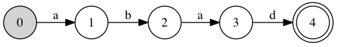
The initial state is in grey, the accept state is a double circle, and transitions are labelled with the character they accept.
Finding the substring “abad” in a long string thus reduces to a bunch of bitwise operations. At each step, we OR bit 0 in the set of states: we’re always looking for the beginning of a new match. Then, we consume a character. If it’s ‘a’, the mask is 0b01010; if it’s ‘b’, mask is 0b00100; if it’s ‘d’, mask is 0b10000; otherwise, its mask is 0. Then, we shift the set of state left by 1 bit, and AND with mask. The effect is that bit 1 is set iff mask has bit 1 set (and that only happens if the character is ‘a’), and bit 0 was previously set (… which is always the case), bit 2 is set iff mask has bit 2 set (i.e. we consumed a ‘b’) and bit 1 was previously set, etc.
We declare victory whenever state 4 is reached, after a simple bit test.
It’s pretty clear that this idea can be extended to wildcards or even character classes: multiple characters can have the same bit set to 1 in their mask. Large alphabets are also straightforward to handle: the mapping from character to mask can be any associative dictionary, e.g. a perfect hash table (wildcards and inverted character classes then work by modifying the default mask value). This works not only with strings, but with any sequence of objects, as long as we can easily map objects to attributes, and attributes to masks. Some thinking shows it’s even possible to handle the repetition operator “+”: it’s simply a conditional transition from state \( i \) to state \( i \).
What I find amazing is that the technique extends naturally to arbitrary regular expressions (or nondeterministic finite automata).
Shift and mask for regular expressions
Simulating an NFA by advancing a set of states in lockstep is an old technique. Russ Cox has written a nice review of classic techniques to parse or recognize regular languages. The NFA simulation was first described by Thomson in 1977, but it’s regularly being rediscovered as taking the Brzozowski derivative of regular expressions ;)
Fast Text Searching With Errors by Sun Wu and Udi Manber is a treasure trove of clever ideas to compile pattern matching, a symbolic task, into simple bitwise operations. For regular expressions, the key insight is that the set of states can be represented with a bitset such that the transition table for the NFA’s states can be factored into a simple data-dependent part followed by \( \epsilon \)-transitions that are the same, regardless of the character consumed. Even better: the NFA’s state can be numbered so that each character transition is from state \( i \) to \( i+1 \), and such a numbering falls naturally from the obvious way to translate regular expression ASTs into NFAs.
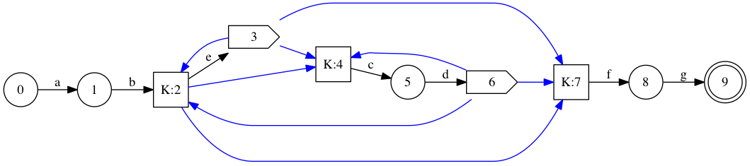
For the initial example “ab(cd|e)*fg”, the AST looks like a node to match ‘a’, succeeded by a node to match ‘b’, then a repetition node into either “cd”, “e” or \( \epsilon \), and the repetition node is succeeded by “fg” (and, finally, accept). Again, a drawing is much clearer!
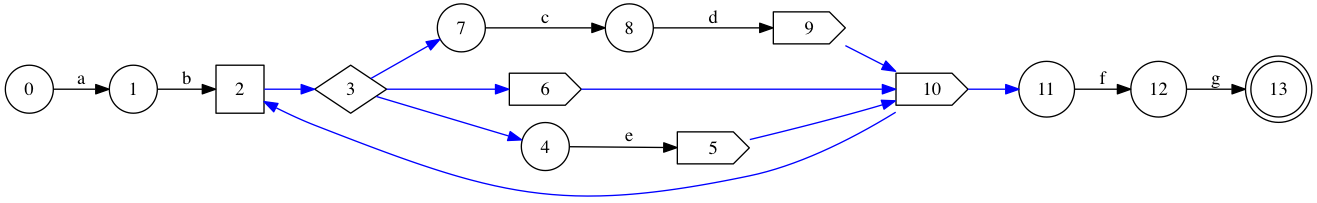
Circles correspond to character-matching states, the square to a repetition node, the diamond to a choice node, and the pointy boxes to dummy states. The final accept state is, again, a double circle. \( \epsilon \)-transitions are marked in blue, and regular transitions are labelled with the character they consume.
The nodes are numbered according to a straight depth-first ordering in which children are traversed before the successor. As promised, character transitions are all from \( i \) to \( i+1 \), e.g. 0 to 1, 1 to 2, 6 to 7, … This is a simple consequence of the fact that character-matching nodes have no children and a single successor.
This numbering is criminally wasteful. States 3, 6 and 10 serves no purpose, except forwarding \( \epsilon \) transitions to other states. The size of the state machine matters because bitwise operations become less efficient when values larger than a machine word must be manipulated. Using fewer states means that larger regular expressions will be executed more quickly.
Eliminating them and sliding the numbers back yields the something equivalent to the more reasonable 11-state machine shown in Wu and Manber (Figure 3 on page 10). Simply not assigning numbers to states that don’t match characters and don’t follow character states suffices to obtain such decent numberings.
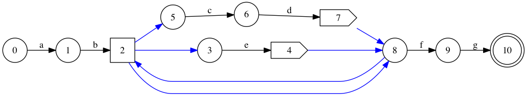
Some more thinking shows we can do better, and shave three more states. State 2 could directly match against character ‘e’, instead of only forwarding into state 3; what is currently state 4 could match against character ‘c’, instead of only forwarding into state 8, then 2 and then 5 (which itself matches against ‘c’); and similarly for state 7 into state 8. The result wastes not a single state: each state is used to match against a character, except for the accept state. Interestingly, the \( \epsilon \) transitions are also more regular: they form a complete graph between states 2, 3 and 5.
It’s possible to use fewer states than the naïve translation, and it’s useful to do so. How can a program find compact numberings?
Compact bitap automata
The natural impulse for functional programmers (particularly functional compiler writers ;) is probably to start matching patterns to iteratively reduce the graph. If they’ve had bad experience with slow fixpoint computations, there might also be some attempts at recognising patterns before even emitting them.
This certainly describes my first couple stabs; they were either mediocre or wrong (sometimes both), and certainly not easy to reason about. It took me a while to heed age-old advice about crossing the street and compacting state machines.

Really, what we’re trying to do when compacting the state machine is to determine equivalence classes of states: sets of states that can be tracked as an atomic unit. With rewrite rules, we start by assuming that all the states are distinct, and gradually merge them. In other words, we’re computing a fixed point starting from the initial hypothesis that nothing is equivalent.
Problem is, we should be doing the opposite! If we assume that all the states can be tracked as a single unit, and break equivalence classes up in as we’re proven wrong, we’ll get maximal equivalence classes (and thus as few classes as possible).
To achieve this, I start with the naïvely numbered state machine. I’ll refer to the start state and character states as “interesting sources”, and to the accept state and character states as “interesting destinations”. Ideally, we’d be able to eliminate everything but interesting destinations: the start state can be preprocessed away by instead working with all the interesting destinations transitively reachable from the start state via \( \epsilon \) transitions (including itself if applicable).
The idea is that two states are equivalent iff they are always active after the same set of interesting sources. For example, after the start state 0, only state 1 is active (assuming that the character matches). After state 1, however, all of 2, 3, 4, 6, 7, 10 and 11 are active. We have the same set after states 4 and 8. Finally, only one state is alive after each of 11 and 12.
Intersecting the equivalence relations thus defined give a few trivial equivalence classes (0, 1, 5, 8, 9, 12, 13), and one huge equivalence class comprised of {2,3,4,6,7,10,11} made of all the states that are active exactly after 1, 5 and 9. For simplicity’s sake, I’ll refer to that equivalence class as K. After contraction, we find this smaller state graph.
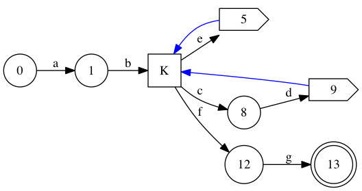
We can renumber this reasonably to obey the restriction on character edges: K is split into three nodes (one for each outgoing character-consuming edge) numbered 2, 4 and 7.
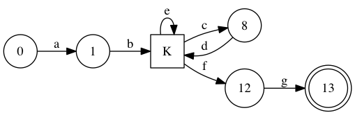
We could do even better if 5 and 9 (3 and 6 above) in the earlier contracted graph were also in equivalence class K: they only exist to forward back into K! I suggest to achieve that with a simple post-processing pass.
Equivalence classes are found by find determining after which interesting node each state is live. States that are live after exactly the same sets of interesting nodes define an equivalence class. I’ll denote this map from state to transitive interesting predecessors \( pred(state) \).
We can coarsen the relationship a bit, to obtain \( pred\sp{\prime}(state) \). For interesting destinations, \( pred\sp{\prime} = pred \). For other nodes, \(pred\sp{\prime}(state) = \cap\sb{s\in reachable(state)}pred(s)\), where \(reachable(state)\) is the set of interesting destinations reachable via \( \epsilon \) transitions from \(state\). This widening makes sense because \(state\) isn’t interesting (we never want to know whether it is active, only whether its reachable set is), so it doesn’t matter if \(state\) is active when it shouldn’t, as long as its destinations would all be active anyway.
This is how we get the final set of equivalence classes.
We’re left with a directed multigraph, and we’d like to label nodes such that each outgoing edge goes from its own label \( i \) to \( i+1 \). We wish to do so while using the fewest number of labels. I’m pretty sure we can reduce something NP-Hard like the minimum path cover problem to this problem, but we can still attempt a simple heuristic.
If there were an Eulerian directed path in the multigraph, that path would give a minimal set of labels: simply label the origin of each arc with its rank in the path. An easy way to generate an Eulerian circuit, if there is one, is to simply keep following any unvisited outgoing arc. If we’re stuck in a dead end, restart from any vertex that has been visited and still has unvisited outgoing arcs.
There’s a fair amount of underspecification there. Whenever many equivalence classes could be chosen, I choose the one that corresponds to the lexicographically minimal (sorted) set of regexp states (with respect to their depth-first numbering). This has the effect of mostly following the depth-first traversal, which isn’t that bad. There’s also no guarantee that there exists an Eulerian path. If we’re completely stuck, I start another Eulerian path, again starting from the lexicographically minimal equivalence class with an unvisited outgoing edge.
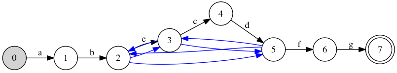
Finally, once the equivalence states are labelled, both character and \( \epsilon \) transitions are re-expressed in terms of these labels. The result is a nice 8-state machine.
But that’s just theory
This only covers the abstract stuff. There’s a
CL code dump on github.
You’re probably looking for compile-regexp3.lisp and
scalar-bitap.lisp; the rest are failed experiments.
Once a small labeling is found, generating a matcher is really straightforward. The data-dependent masks are just a dictionary lookup (probably in a vector or in a perfect hash table), a shift and a mask.
Traditionally, epsilon transitions have been implemented with a few
table lookups. For example, the input state can be cut up in bytes;
each byte maps to a word in a different lookup table, and all the
bytes are ORed together. The tables can be pretty huge (n-states/8
lookup tables of 256 state values each), and the process can be slow
for large states (bitsets). This makes it even more important to
reduce the size of the state machine.
When runtime compilation is easy, it seems to make sense to instead generate a small number of test and conditional moves… even more so if SIMD is used to handle larger state sets. A couple branch-free instructions to avoid some uncorrelated accesses to LUTs looks like a reasonable tradeoff, and, if SIMD is involved, the lookups would probably cause some slow cross-pipeline ping-ponging.
There’s another interesting low-level trick. It’s possible to handle large state sets without multi-word shifts: simply insert padding states (linked via \( \epsilon \) transitions) to avoid character transitions that straddle word boundaries.
There’s a lot more depth to this bitap for regexp matching thing. For example, bitap regular expressions can be adapted to fuzzy matchings (up to a maximum edit distance), by counting the edit distance in unary and working with one bitset for each edit distance value. More important in practice, the approach described so far only handles recognising a regular language; parsing into capture groups and selecting the correct match is a complex issue about which Russ Cox has a lot to say.
What I find interesting is that running the NFA backward from accept states gives us a forward oracle: we can then tell whether a certain state at a given location in the string will eventually reach an accept state. Guiding an otherwise deterministic parsing process with such a regular language oracle clearly suffices to implement capture groups (all non-deterministic choices become deterministic), but it also looks like it would be possible to parse useful non-regular languages without backtracking or overly onerous memoisation.