TL;DR: Optimisers compose, satisfiers don’t.

One rainy day at Sophia-Antipolis, a researcher told me a story about an optimisation software company. They’d looked into adding explicit support for Dantzig-Wolfe decomposition, but market research showed there were a few hundred potential users at most: too few people are familiar enough with decomposition methods to implement new ones. The problem is, the strength of these methods is that they are guided by domain expertise; useful decompositions are custom-made for the target problem, and thus obviously novel. What this story tells me is that we, researchers in decomposition, are really bad communicators.

It’s not like these methods are new or ill understood. The theory on how to break up optimisation problems into smaller ones (for Benders and Dantzig-Wolfe decompositions, at least) was fully developed in the fifties and sixties. It’s the same theory that backs state-of-the-art solvers for planet-scale planning problems today. Surprisingly, it seems that a single undergraduate or graduate course in optimisation methods does not suffice for expertise to trickle down to the wider computer science and management communities.

The divide seems particularly wide with the constraint programming (CP) community (despite the work of Hooker, Chvátal and Achterberg [that I know of]). Perhaps this explains why the VPRI’s efforts on cooperating constraint solvers are not informed by decomposition methods at all. Then again, it’s not just decomposition people who exchange too little with the CP community, but all of mathematical programming. I only single out decomposition because our tools are general enough to work with CP. We write and sometimes think in mixed integer linear programming (MILP) terms, but mostly for theoretical reasons; implementations may (useful ones usually do) include specialised solvers for combinatorial problems that only happen to be presented as MILP.

That’s why I spent three months in Nice: I explored how to cross-pollinate between CP and decomposition by developing a TSP solver (it’s a simple problem and Concorde is an impressive baseline). I have a lot to say about that, certainly more than can fit in this buffer. In this first post of many, I hope to communicate an intuition on why Dantzig-Wolfe and Benders decomposition work, to relate these methods to work from the SAT/CSP/CP community, and to show how to decompose finite domain problems.

But first, duality

I noted earlier that we work in MILP terms because it gives a sound theoretical basis for decomposition methods. That basis is duality, especially linear programming duality.

In optimisation, duality refers to the relationship between two problems a primal problem (P) and its dual (D). I’ll assume that we’re interested in solving (P), a minimisation problem (minimise badness, e.g., costs); (D) is then a maximisation problem (maximise goodness, e.g., profits). These problems are such that the minimal (least) value for (P) is always higher or equal to the maximal (greatest) value for (D).

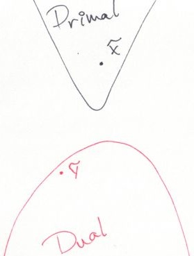
So, even if (P) and (D) are so hard that we can only solve them heuristically, a pair of feasible solutions always brackets the optimal value for the primal problem (P). \(\tilde{x}\), the feasible solution for (P) might not be optimal, but it’s still a solution. In turn, \(\tilde{y}\), the dual feasible solution, gives us a lower bound on the optimal value: we don’t know the optimal value, but we know it can’t be lower than that of any solution for (D). We can then compare the value of \(\tilde{x}\) to this lower bound. If they’re close enough, we stop looking; otherwise we use both primal and dual information to refine our solutions and tighten the bracket (close the gap).

The primal solution is useful: it’s a feasible plan. However, the dual solution is often where we gain insights into the problem. For example, if I wish to minimise my carbon footprint, it’s clear that driving less will help me. However, what is the impact of allowing myself more commuting time? and how does that compare with simply shortening the distance between my home and work? That’s what dual solutions tell us: they estimate the impact of (the right-hand side of) each constraint on the objective value.

Linear programs are a special case: they have a “strong” duality, in that we can easily write down an exact dual program for any primal linear program. The dual is exact because its maximal value matches the minimal value of the primal; there is no duality gap. This dual is another linear program that’s exactly as large as the primal, and the dual of the dual is… the initial primal program.

Decomposition exploits this relationship to extract information about simpler subproblems, and translate that into a refined approximation of the complete problem. It would be disappointing if that only worked on linear programs, and this is where Lagrangian duality comes in.

You may remember Lagrange multipliers from calculus courses. That’s exactly what I’m talking about. For reasons both practical and theoretical, I’ll assume that we have a (sub)problem that’s simpler once a few linear (affine) constraints are removed, i.e. something like \(\min\sb{x} z(x)\) subject to \(Ax \leq b,\) \(x\in X.\)

This form is general; the objective function \(z\) need only be convex and the feasible set \(X\) is arbitrary.

Lagrangian duality says that we can relax this problem into \(\min\sb{x\in X} z(x) + \lambda(Ax-b),\) where \(\lambda\) is any vector of non-negative multipliers for each row (constraint) in \(A\). I find such subproblems interesting because minimising over \(X\) can be easy with a specialised procedure, but hard as a linear program. For example, \(X\) could represent spanning trees for a graph. That’s how the one-tree relaxation for the TSP works. Once you remove an arbitrary “one-node” from a Hamiltonian cycle, the remaining Hamiltonian path is a special kind of spanning tree: the degree of all but two nodes is two, and the remaining two nodes are endpoints (would be connected to the one-node). The one-tree relaxation dualises (relaxes into the objective function) the constraint that the degree of each node be at most two, and solves the remaining minimum spanning tree problem for many values of \(\lambda\).

The one-tree subproblem, and Lagrangian subproblems in general, is a relaxation because any optimal solution to this problem is a lower bound for the optimal value of the initial problem.

To show this, we first notice that the feasible set of the subproblem is a superset of that of the initial problem: we only removed a set of linear constraints. Moreover, for any feasible solution \(\bar{x}\) for the initial problem, \(z(\bar{x}) + \lambda(A\bar{x}-b) \leq z(\bar{x}):\) \(A\bar{x} \leq b\), i.e., \(A\bar{x}-b \leq 0\), and \(\lambda\geq 0\). In particular, that is true if \(\bar{x}\) is an optimal solution to the initial problem. Obviously, an optimal solution to the relaxed subproblem must be at least as good as \(\bar{x}\), and the optimal value of the subproblem is a lower bound for that of the initial problem.

This relation between optimal solutions for the initial problem and for the relaxed subproblem is true given any \(\lambda\geq 0\). However, it’s often useless: bad multipliers (e.g., \(\lambda = 0\)) lead to trivially weak bounds. The Lagrangian dual problem with respect to \(Ax \leq b\) is to maximise this lower bound: \(\max\sb{\lambda\geq 0} \min\sb{x\in X} F(\lambda, x),\) where \(F(\lambda, x) = z(x) + \lambda(Ax-b) = z(x) + \lambda Ax - \lambda b.\)

Again, we don’t have to maximise this dual exactly. As long as the minisation subproblem is solved to optimality, we have a set of lower bounds; we only have to consider the highest lower bound. Maximising this Lagrangian dual, given an oracle that solves the linearly penalised subproblem, is an interesting problem in itself that I won’t address in this post. The important bit is that it’s doable, if only approximately, even with very little storage and computing power.

There’s some nifty theoretical results that tell us that, when \(z(x)\) is a linear function, maximising the Lagrangian dual function is equivalent to solving the linear programming dual of \(\min z(x)\) subject to \(Ax \leq b,\) \(x\in \textrm{conv}(X),\) where \(\textrm{conv}(X)\) is the convex hull of \(X\).

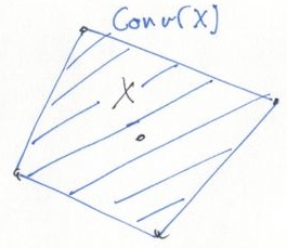
This is a relaxation (the convex hull is superset of \(X\)), but a particularly tight one. For example, if \(X\) is a finite set, optimising a linear function over \(\textrm{conv}(X)\) is equivalent to doing so over \(X\) itself. Sadly, this doesn’t hold anymore once we add the linear constraint \(Ax \leq b\) after taking the convex hull, but still gives an idea of how strong the relaxation can be.

One key detail here is that the optimality of \(x\) depends on \(\lambda\), \(z\), \(X\) and \(A\), but not on \(b\): once we have a pair \((\lambda\sp{\star}, x\sp{\star})\) such that \(x\sp{\star}\) is minimal for \(F(\lambda\sp{\star},\cdot)\), their objective value is always a valid lower bound for the initial problem, regardless of the right-hand side \(b\). Thus, it make sense to cache a bunch of multiplier-solution pairs: whenever \(b\) changes, we only need to reevaluate their new objective value to obtain lower bounds for the modified problem (and interesting pairs can serve to warm start the search for better maximising multipliers).

Intermission

Why optimisation, when satisfaction is hard enough?

Because I’m a heartless capitalist. (I find it interesting how economists sometimes seem overly eager to map results based on strong duality to the [not obviously convex] world.)

Seriously, because optimisation composes better than satisfaction. For example, imagine that we only had a routine to enumerate elements of \(X\). There’s not a lot we can do to optimise over \(X\) (when you seriously consider a British Museum search…), or even just to determine if the intersection of \(X\) and \(Ax \leq b\) is empty.

I’ve hinted as to how we can instead exploit an optimisation routine over \(X\) to optimise over an outer approximation of that intersection. It’s not exact, but it’s often close enough; when it isn’t, that approximation is still useful to guide branch-and-bound searches. A satisfaction problem is simply an optimisation problem with \(z(x) = 0\). Whenever we have a relaxed solution with a strictly positive objective value, we can prune a section of the search space; at some point we either find a feasible solution or prune away all the search space. Thus, even for pure satisfaction problems, the objective function is useful: it replaces a binary indicator (perhaps feasible, definitely infeasible) with a continuous one (higher values for less clearly feasible parts of the search space).

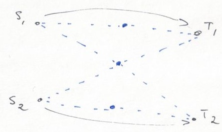
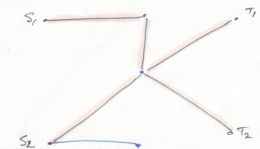
I said optimisation composes better because decomposition also works for the intersection of sets defined by oracles. For example, we can satisfy over the intersection of finite sets \(X\) and \(Y\) by relaxing the linear constraint in \(x = y,\) \(x\in X, y\in Y.\) The relaxed subproblem is then \(\min\sb{(x,y)\in X\times Y} \lambda(x-y),\) which we can separate (linear objectives are separable) into two optimisation subproblems: \(\min\sb{x\in X} \lambda x,\) and \(\min\sb{y\in Y} -\lambda y.\) Even if the initial problem is one of satisfaction, Lagrangian decomposition considers each finite set in the intersection through independent minimisation: components communicate via their objective functions.

But I don’t deal with numbers

All this can also work with categorical data; we just have to do what no CP practicioner would ever do and map each choice to a binary (0/1) variable. When, in the constraint program, a variable \(x\) can take values \({a, b, c}\), we express that in integer programs with a triplet of variables:

• \(x\sb{a} = 1\) iff \(x=a\) (0 otherwise),
• \(x\sb{b} = 1\) iff \(x=b\),
• \(x\sb{c} = 1\) iff \(x=c\),

and a constraint \(\sum\sb{i\in {a,b,c}} x\sb{i} = 1\).

We can perform this mapping around each subproblem (e.g., optimisation over \(X\)). On entry, the coefficient for \(x\sb{a}\) in the linear objective corresponds to the impact on the objective function of letting \(x=a\). On exit, \(x=c\) becomes \(x\sb{c}=1\), \(x\sb{a}=0\) and \(x\sb{b}=0\), for example.

Benders decomposition

Benders decomposition is the mathematical programming equivalent of clause learning in SAT solvers, or explanation-based search in CP.

Clause learning improves straight backtracking by extracting information from infeasible branches: what’s a small (minimal is NP-hard) set of assignments (e.g. \(x=\mathtt{false}\) and \(y=\mathtt{false}\)) that causes this infeasibility? The problem is then updated to avoid this partial assignment.

Explanations in CP are similar: when a global constraint declares infeasibility, it can also provide an explanation, a small set of assignments that must be avoided. This, combined with explanations from other constraints, can trigger further propagation.

Benders decomposition generalises this feasibility-oriented view for the optimisation of problems with a hierarchical structure. I think the parallel has been known for a while, just not popularised. John Hooker proposed logic-based Benders to try and strengthen the link with logic programming, but I don’t know who (if anyone) else works in that direction.

The idea behind Benders decomposition is to partition the decision variables in two sets, strategic variables \(y\), and tactical ones \(x\). The decomposition attempts to determine good values for \(y\) without spending too much time on \(x\), which are left for the subproblem. This method is usually presented for mixed integer programs with continuous tactical (\(x\)) variables, but I’ll instead present the generalised form, which seems well suited to constraint programming.

We start with the initial integrated formulation \(\min\sb{(x,y)\in S} cx + fy,\) which we reformulate as \(\min\sb{(x,y)} cx + fy,\) \(y\in Y,\) \(x\in X(y).\)

For example, this could be a network design problem: we wish to determine where to build links so that all (known) communication demands are satisfied at least total cost.

Benders decomposition then eliminates variables \(x\) from the reformulation. The latter becomes the master problem \(\min\sb{y,z} fy + z\) subject to \(Ay = d,\) \(By \leq z,\) \(y\in Y.\)

The two linear constraints are generated dynamically, by solving subproblems over \(X\). The first corresponds directly to learned clauses or failure explanations: whenever an assignment for \(y\) happens to be infeasible, we add a linear constraint to avoid it (and similar assignments) in the future. The second enables optimisation over \(S\).

The idea is to solve a Lagrangian relaxation of the (slave) subproblem for a given assignment \(y\sp{i}\): \(\min\sb{x,y} cx\) subject to \(y = y\sp{i},\) \(x\in X(y).\)

We will relax the first equality constraint to obtain a new feasible set that is a relaxation (outer approximation) of \(S\): it only considers interactions within \(X\) and between \(X\) and \(Y\), but not within \(Y\) (those are handled in the master problem).

In my network design example, the unrelaxed subproblem would be a lot of independent shortest path problems (over the edges that are open in \(y\sp{i}\)).

We dualise the first constraint and obtain the Lagrangian dual \(\max\sb{\lambda} \min\sb{y\in\mathbb{R}\sp{m}, x\in X(y)} cx + \lambda(y-y\sp{i})\) or, equivalently, \(\max\sb{\lambda} -\lambda y\sp{i} + \min\sb{y\in\mathbb{R}\sp{m}, x\in X(y)} cx + \lambda y.\)

The network design subproblem still reduces to a lot of independent shortest path problems, but (with appropriate duplication of decision variables) forbidden edges may be taken, at additional cost per flow.

In this example, the previous step is gratuitously convoluted: we can solve the unrelaxed subproblem and shortest paths can be seen as linear programs, so there are other ways to recover optimal multipliers directly. However, this is useful for more complicated subproblems, particularly when the \(x = y\sp{i}\) constraint is difficult to handle. Note that the slave can be reformulated (e.g., with multiple clones of \(y\sp{i}\)) to simplify the Lagrangian subproblem.

I pointed out earlier that, given \(\bar{\lambda}\sp{i}\) and an optimal solution \((\bar{x}\sp{i},\bar{y}\sp{i})\) for that vector of multipliers, we always have a valid lower bound, regardless of the right-hand side, i.e., regardless of the assignment \(y\sp{i}\).

We found a first (hopefully feasible) solution by solving a restricted subproblem in the previous step. The multipliers for our dualised constraint \(y = y\sp{i}\) explain the value associated to \(y\sp{i}\), what part of \(y\sp{i}\) makes the solution to the restricted subproblem so bad (or good).

That’s how we dynamically constrain \(z\). Each time we solve the (updated) master problem, we get a tentative assignment for the strategic variables, and a lower bound for the initial problem. We can then solve for \(x\in X(y\sp{i})\) to find a heuristic solution (or generate a feasibility cut to tell the master why the assignment is infeasible); if the heuristic solution is close enough to our current lower bound, we can stop the search. Otherwise, we solve the fixed Lagrangian dual and generate a fresh optimality cut \(-\bar{\lambda}\sp{i}y + c\sp{i} \leq z,\) where \(c\sp{i} = c\bar{x}\sp{i} + \bar{\lambda}\sp{i}\bar{y}\sp{i}\): we update the master problem with information about why its last tentative assignment isn’t as good as it looked.

It can be harder to explain infeasibility than to solve the Lagrangian subproblem. In that case, it suffices to have an upper bound on the optimal value (e.g., 0 for pure feasibility problems): when the lower bound is greater than the upper bound, the problem is infeasible. Given that the master problem also tries to minimise its total cost, it will avoid solutions that are infeasible if only because their value is too high. The advantage of feasibility cuts is that, with some thinking, a single feasibility cut can forbid a lot more solutions than multiple optimality cuts.

The problem with Benders decomposition is that the master mixed integer program gains new constraints at each iteration. Eventually, its size becomes a liability.

There are a few folk workarounds. One is to not stop (and then restart) the branch-and-bound search as soon as it finds an optimal (for the current relaxed master problem) integer feasible assignment for \(y\): instead, add a new constraint to the formulation and resume the search (previously computed lower bounds remain valid when we add constraints). Another is to drop constraints that have been inactive for a long while (much like cache replacement strategies); they can always be added back if they ever would be active again.

Chvátal’s Resolution Search takes a different tack: it imposes a structure on the clauses it learns to make sure they can be represented compactly. The master problem is completely different and doesn’t depend on solving mixed integer programs anymore. It works well on problems where the difficulty lies in satisfying the constraints more than finding an optimal solution. A close friend of mine worked on extensions of the method, and it’s not yet clear to me that it’s widely applicable… but there’s hope.

Another issue is that the Benders lower bound is only exact if the slave subproblem is a linear program. In the general case, the master problem is still useful, as a lower bounding method and as a fancy heuristic to guide our search, but it may be necessary to also branch on \(x\) to close the gap.

Lagrangian decomposition

I believe Lagrangian decomposition, a special case of Lagrangian relaxation, is a more promising approach to improve constraint programming with mathematical programming ideas: I think it works better with the split between constraint propagation and search. The decomposition scheme helps constraints communicate better than via only domain reductions: adjustments to the objective functions pass around partial information, e.g., “\(x\) is likely not equal to \(a\) in feasible/optimal solutions.” Caveat lector, after 7 years of hard work, I’m probably biased (Stockholm syndrome and all that ;).

I already presented the basic idea. We take an initial integrated problem \(\min\sb{x\in X\cap Y} cx\) and reformulate it as \(\min\sb{(x,y)\in X\times Y} cx\) subject to \(x = y.\) Of course, this works for any finite number of sets in the intersection as well as for partial intersections, e.g., \(x\sb{0} = y\sb{0}\) and \(x\) and \(y\) otherwise independent.

Dualising the linear constraint leaves the independent subproblems \(\min\sb{x\in X} cx+\lambda x,\) and \(\min\sb{y\in Y} -\lambda y.\)

The two subproblems communicate indirectly, through adjustments to \(\lambda\)… and updating Lagrange multipliers is a fascinating topic in itself that I’ll leave for a later post (: The basic idea is that, if \(x\sb{i} = 1\) and \(y\sb{i} = 0\), we increase the associated multiplier \(\lambda\sb{i}\), and decrease it in the opposite situation: the new multipliers make the current incoherence less attractive. For a first implementation, subgradient methods (e.g., the volume algorithm) may be interesting because they’re so simple. In my experience, however, bundle methods work better for non-trivial subproblems.

When we have an upper bound on the optimal value (e.g., 0 for pure satisfaction problems), each new multipliers \(\lambda\) can also trigger more pruning: if forcing \(x = a\) means that the lower bound becomes higher than the known upper bound, we must have \(x \neq a\). The challenges becomes to find specialised ways to perform such pruning (based on reduced costs) efficiently, without evaluating each possibility.

Lagrangian decomposition also gives us a fractional solution to go with our lower bound. Thus, we may guide branching decisions with fractional variables, rather than only domains. Again, an optimisation-oriented view augments the classic discrete indicators of CP (this variable may or may not take that value) with continuous ones (this assignment is unattractive, or that variable is split .5/.5 between these two values).

Hybrid mathematical/constraint programming

I believe decomposition methods are useful for constraint programming at two levels: to enable more communication between constraints, and then to guide branching choices and heuristics.

In classic constraint programming, constraint communicate by reducing the domain of decision variables. For example, given \(x \leq y\), any change to the upper bound for \(y\) (e.g., \(y\in [0, 5]\)) means that we can tighten the upper bound of \(x\): \(x \leq y \leq 5\). This can in turn trigger more domain reduction.

Some constraints also come in “weighted” version, e.g., \(x\sb{i}\) form a Hamiltonian cycle of weight (cost) at most 5, but these constraints still only communicate through the domain of shared decision variables.

With Lagrangian decomposition, we generalise domain reduction through optimisation and reduced cost oracles. For each constraint, we ask, in isolation,

• to the optimisation oracle: given this linear objective function for the variables that appear in the constraint, what’s an optimal solution?
• to the reduced cost oracle: given this objective function and optimal solution, what’s the impact (or a lower estimate of that impact, a reduced cost) on the objective value of forcing each variable to a different value?

Adding the objective values computed by the optimisation oracle gives us a lower bound. If the lower bound is greater than some upper bound, the problem (search node) is infeasible. Otherwise, we can use reduced costs to prune possibilities.

Let’s say the difference between our current lower and upper bounds is \(\Delta\). We prune possibilities by determining whether setting \(x=a\) increases the lower bound by more than \(\Delta\). We can do this independently for each constraint, or we can go for additive bounding. Additive bounding computes a (lower) estimate for the impact of each assignment on the objective function, and sums these reduced costs for all constraints. The result is a set of valid lower estimates for all constraints simultaneously. We can then scan these reduced costs and prune away all possibilities that lead to an increase that’s greater than \(\Delta\).

The optimisation oracle must be exact, but the reduced cost oracle can be trivially weak (in the extreme, reduced costs are always 0) without affecting correctness. Domain reduction propagators are simply a special case of reduced cost oracles: infeasible solutions have an arbitrarily bad objective value.

Some constraints also come with explanations: whenever they declare infeasibility, they can also generate a small assignment to avoid in the future. The mathematical programming equivalent is cut generation to eliminate fractional solutions. Some very well understood problems (constraints) come with specialised cuts that eliminate fractional solutions, which seems useful in hybrid solvers. For example, in my work on the TSP, I added the (redundant) constraint that Hamiltonian cycles must be 2-matchings. Whenever the Lagrangian dual problem was solved fairly accurately, I stopped to compute a fractional solution (for a convexification of the discrete feasible set) that approximately met the current lower bound. I then used that fractional solution to generate new constraints that forbid fractional 2-matchings, including the current fractional solution. These constraints increased the lower bound the next time I maximised the Lagrangian dual, and thus caused additional reduced cost pruning.

The same fractional solution I used to generate integrality cuts can also guide branching. There’s a lot of interesting literature on branching choices, in CP as well as in mathematical programming. Lagrangian decomposition, by computing fractional solutions and lower bounds, let us choose from both worlds. Again, the lower bound is useful even for pure feasibility problems: they are simply problems for which we have a trivial upper bound of 0, but relaxations may be lower. Only branching on fractional decision variables also let us cope better with weak domain propagators: the relaxation will naturally avoid assignments that are infeasible for individual constraints… we just can’t tell the difference between a choice that’s infeasible or simply uninteresting because of the objective function.

Automated CP decomposition

This is a lot more tentative than everything above, but I believe that we can generate decomposition automatically by studying (hyper)tree decompositions for our primal constraint graphs. Problems with a small (hyper)treewidth are amenable to quick dynamic programming, if we explore the search space in the order defined by the tree decomposition: a small treewidth means that each subtree depends on a few memoisation keys, and there are thus few possibilities to consider.

For example, I’m pretty sure that the fun poly-time dynamic programming algorithms in the Squiggol book all correspond to problems with a bounded tree-width for the constraint graph.

In general though, problems don’t have a small treewidth. This is where mathematical decomposition methods come in. Benders decomposition could move a few key linking variables to the master problem; once they are taken out of the slave subproblem, the fixed Lagrangian subproblem has a small tree width.

However, I already wrote that Lagrangian decomposition seems like a better fit to me. In that case, we find a few variables such that removing them from the primal graph leaves a small tree decomposition. Each subproblem gets its own clones of these variables, and Lagrangian decomposition manipulates the objective function to make the clones agree with one another.

With this approach, we could also automatically generate dynamic programming solvers for Lagrangian subproblems… and it might even be practical to do the same for reduced cost oracle.

Going to hypertree-width improves our support for global constraints (e.g., alldiff) or constraints that otherwise affect many variables directly. Global constraint should probably get their own decomposition component, to easily exploit their pruning routines, but not necessarily large ad hoc ones. Hypertree decomposition takes the latter point into account, that a large clique created by a single constraint is simpler to handle than one that corresponds to many smaller (e.g., pairwise) constraints.

What’s next?

I don’t know. I won’t have a lot of time to work on this stuff now that I have a real job. I’ve decided to dedicate what little time I have to a solver for Lagrangian master problems, because even the research community has a bad handle on that.

For the rest, I’m mostly unexcited about work that attempts to explore the search space as quickly as possible. I believe we should instead reify the constraint graph as much as possible to expose the structure of each instance to analyses and propagators, and thus reduce our reliance on search.

As a first step, I’d look into a simple system that only does table constraints (perhaps represented as streams of feasible tuples). A bucket heuristic for tree decomposition may suffice to get decent dynamic programming orders and efficiently optimise over the intersection of these table constraints. (Yes, this is highly related to query optimisation; constraint programming and relational joins have much in common.)

After that, I’d probably play with a few externally specified decomposition schemes, then add support for global constraints, and finally automatic decomposition.

All in all, this looks like more than a thesis’s worth of work…