Implicit data structures are data structures with negligible space overhead compared to storing the data in a flat array: auxiliary information is mostly represented by permuting the elements cleverly. For example, a sorted vector combined with binary search is an implicit in-order representation of a binary search tree. I believe the seminal implicit data structure is the binary heap of Williams and Floyd, usually presented in the context of heapsort.

I find most developers are vastly more comfortable dealing with pointer-based data structures than with implicit ones. I blame our courses, which focus on the former and completely fail to show us how to reason about the latter. For example, the typical presentation of the binary heap introduces an indexing scheme to map from parent to children – the children of heap[i] are heap[2 * i] and heap[2 * i + 1], with one-based indices – that is hard to generalise to ternary or k-ary heaps (Knuth’s presentation, with parents at \(\lfloor i/2 \rfloor\), is no better). The reason it’s so hard to generalise is that the indexing scheme hides a simple bijection between paths in k-way trees and natural numbers.

I find it ironic that I first encountered the idea of describing data structures or algorithms in terms of number systems, through Okasaki’s and Hinze’s work on purely functional data structures: that vantage point seems perfectly suited to the archetypal mutable data structure, the array! I’ll show how number systems help us understand implicit data structures with two examples: a simple indexing scheme for k-ary heaps and compositions of specially structured permutations to implement in-place bit-reversal and (some) matrix transpositions.

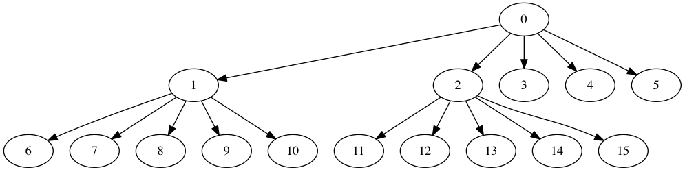
Simple k-ary max heaps

The classical way to present implicit binary heaps is to work with one-based array indices and to root an implicit binary tree at heap[1]. For any node heap[i], the children live at heap[2 * i] and heap[2 * i + 1]. My issue with this presentation is that it’s unclear how to extend the scheme to ternary or k-ary trees: if the children of heap[1] are heap[3 * 1 ... 3 * 1 + 2], i.e., heap[3, 4, 5], what do we do with heap[2]? We end up with k - 1 parallel k-ary trees stashed in the same array. Knuth’s choice of mapping children to parents with a floored integer division suffers the same fate.

One-based arrays hides the beauty of the binary indexing scheme. With zero-based arrays, the children of heap[i] are heap[2 * i + 1] and heap[2 * i + 2]. This is clearly isomorphic to the one-based scheme for binary heaps. The difference is that the extension to k-way trees is obvious: the children of heap[i] are heap[k * i + 1 ... k * i + k].

A couple examples like the one below fail to show any problem. However, even a large number of tests is no proof. Thinking in terms of number systems leads to a nice demonstration that the scheme creates a bijection between infinite k-ary trees and the naturals.

There is a unique finite path from the root to any vertex in an infinite k-ary tree. This path can be described as a finite sequence \((c\sb{1}, c\sb{2}, \ldots, c\sb{n})\) of integers between 1 and k (inclusively). If \(c\sb{1} = 1\), we first went down the first child of the root node; if \(c\sb{1} = 2\), we instead went down the second child; etc. If \(c\sb{2} = 3\), we then went down the third child, and so on. We can recursively encode such finite paths as naturals (in pidgin ML):

path_to_nat [] = 0
path_to_nat [c : cs] = k * path_to_nat cs + c

Clearly, this is an injection from finite paths in k-ary trees to the naturals. There’s only a tiny difference with the normal positional encoding of naturals in base k: there is no 0, and digits instead include k. This prevents us from padding a path with zeros, which would map multiple paths to the same natural.

We only have to show that path_to_nat is a bijection between finite paths and naturals. I’ll do that by constructing an inverse that is total on the naturals.

nat_to_path 0 = []
nat_to_path n = let c = pop n
                in c : nat_to_path (n - c) / k

where pop is a version of the mod k that returns k instead of 0:

pop n = let c = n `mod` k
        in 
         if (c != 0)
          then c
          else k

The base case is nat_to_path 0 = [].

In the induction step, we can assume that path_to_nat cs = n and that nat_to_path n = cs. We only have to show that, for any \(1 \leq c \leq k\), nat_to_path path_to_nat c:cs = c:cs. Let n' = path_to_nat c:cs = k * n + c.

\[n\sp{\prime} = kn + c \equiv c\quad \mod k,\] so pop n' will correctly return c (and k rather than 0). It’s then a tiny bit of algebra to show that (n' - c) / k = n, and we fall back to the induction hypothesis.

This scheme is so simple that I wound up coding a version of heapsort(3) that lets callers choose the heap’s arity at runtime. Higher arity heaps perform more comparisons but fewer swaps than binary heaps; the tradeoff is profitable when sorting large items. It seems to me that, for decades, we’ve been presenting implicit heaps and heapsort in a way that marginally simplifies the binary case at the expense of obscuring the elegant general case.

Array permutations as algebra on positional number systems

Bit reversing an array of length \(2\sp{l}\) sends the element x[i] to x[j], where the binary representation of i (including padding up to l bits) is the reverse of j. For example, in an array of length 16, 3 = 0011 becomes 1100 = 12.

Reversing a fixed-width integer’s binary representation is its self-inverse, so bit reversing an array is a sequence of swaps. This means that the permutation can be performed in-place, as a series of independent swaps. Bit reversal used to be slow on cached machines: contiguous elements (with indices that only vary in their low order bits) swap with far-off elements (indices that only vary in their high order bits). Worse, the stride between the latter elements is a large power of two, which causes all sorts of aliasing issues. Workarounds (see Zhang 99 (PDF)) mostly end up implementing a software cache with explicit buffers. Nowadays, even L1 caches have such a high associativity that aliasing is a much less important issue.

Napa-FFT3 implements bit reversals by calling a few specialised functions that only swap the lower and higher bits; the main routine iterates over an array of precomputed middle bit reversals (similar to various publications of Elster’s, but recursing on the middle bits first). In this implementation, the number of L1 cache misses incurred by bit reversing an array is only slightly greater than the compulsory misses. Bit reversal isn’t free, but it’s also not clear that autosorting FFTs are quicker than out-of-order FFTs followed by a bit reversal pass.

Bit reversal is the only array permutation I’ve seen described in terms of its effect on indices. I think it’s a fruitful avenue for other in-place permutations.

For example, the viewpoint makes it clear how to transpose a matrix of dimensions \(2\sp{m} \times 2\sp{n}\) with a sequence of in-place bit reversals (each \(i\sb{k}\) and \(j\sb{l}\) is a bit in the index’s binary representation).

For a row-major layout, the sketch above corresponds to:

1. bit reverse each row of length \(2\sp{n}\) in place;
2. bit reverse the whole vector of length \(2\sp{m + n}\) in place;
3. bit reverse each new row of length \(2\sp{m}\) in place.

Bit reversal, like all other permutations, is a reversible linear operation. We can thus change the order of operation if we want to. For example, it’s not necessarily preferable to bit-reverse contiguous rows first. We could also flip the high-order bits of the indices: rather than swapping scalars, we would swap rows. Separately bit reversing contiguous rows works best when each row fits in cache. Bit reversing columns instead amortises the bad access pattern inherent to bit reversal by spending more time on each swap: swapping rows is slower than swapping scalars, but also very efficients with regards to (streaming!) I/O.

This is interesting because in-place transposition of rectangular matrices is hard, and transposition is already a bad fit for caches. Transposing matrices with a sequence of bit reversals might just be practical. In fact, that’s what I intend to do in Napa-FFT3 for multi-dimensional DFTs: we can fuse all but the middle whole-vector bit reversal with mixed-radix FFTs (and the latter might similarly benefit from operating on [sub-]rows rather than scalars).

One obvious question now appears: can we generalise the trick to general dimensions? It’s pretty clear that we can do it for any other base \(b\) and matrices of dimension \(b\sp{m} \times b\sp{n}\) (it’s interesting how highly composite numbers dimensions are easy to transpose, and, IIRC, so are coprime ones). What if there’s no such factorisation? The best I can do is “more or less.”

For arbitrary matrix dimensions \(m \times n\), I think it’s best to decompose indices in a mixed radix (but still positional) number system. For example, a \(63 \times 21\) matrix might have indices in radix \(3,7\ |\ 3,7,3\). Given this number system, matrix transposition is

It’s a small generalisation to let the radices be \(a,b\ |\ a,b,a\), for a matrix of dimension \(ab \times a\sp{2}b\). We can then perform most of a matrix transposition by swapping positions of identical weight: first a full mixed-radix digit reversal (the weights are palindromic), followed by another mixed-radix reversal on the first three positions.

This leaves the last chunk \(b\sb{2},a\sb{3}\), which should instead be \(a\sb{3},b\sb{2}\). That’s another rectangular matrix tranpose, but smaller than the original one. It might be practical to execute that last step with a straightforward out-of-place transpose: a smaller transpose needs less scratch space and may fit in cache. We can also apply the same trick as for bit reversals and apply the transpose before everything else, by permuting rows rather than scalars. The simplest way to do that is to transpose a matrix of pointers before replicating the permutation on the actual data (glibc’s mergesort references Knuth vol. 3, exercise 5.2-10).

Finally, this also works for \(a\sp{2}b \times ab\): matrix transposition is its own inverse, so we only have execute the inverse of each step, in reverse order.

Definitely mixed results, but at least we have some intuition on why general rectangular transpositions are hard to perform in place: they’re hard to express as sequences of swaps.

Next: C code and cycle counts!

This post is the more theoretical prologue to a low-level look at qsort(3): I really wanted to make sure the nice implicit tree layout in the first section had the space it deserves.

I tried to make in-order implicit trees fit in this number system approach. I can’t see how. The problem is that in-order trees associate ranges (rather than indices) with nodes; for example, at what depth is index 1000? It depends on the size of the search tree. It might be the root (in a tree of 2000 vertices) or a leaf (in a tree of 1001 vertices).