I’m trying something new this week: gathering a small group after work for 90 minutes of short talks and discussions. We’ll also have one longer slot because not everything fits in a postcard, but my main goal is really to create opportunities for everyone to infect us with their excitement for and interest in an idea or a question. I successfully encouraged a couple people to present, although many seemed intimidated by the notion… perhaps because we have grown to expect well researched and rehearsed performances. However, I believe that simple presentations of preliminary work are worthwhile, and probably more likely to spark fresh conversations than the usual polished fare: it’s healthy to expose our doubts, trials, and errors, and there’s certainly value in reminding ourselves that everyone else is in that same boat.

Here’s what I quickly (so quickly that my phone failed to focus correctly) put together on embedding search trees in sorted arrays. You’ll note that the “slides” are very low tech; hopefully, more people will contribute their own style to the potluck next time (:

I didn’t really think about implementing search trees until 3-4 years ago. I met an online collaborator in Paris who, after a couple G&T, brought up the topic of “desert island” data structures: if you were stuck with a computer and a system programming guide on a desert island, how would you rebuild a standard library from scratch? Most data structures and algorithms that we use every day are fairly easy to remember, especially if we don’t care about proofs of performance: basic dynamic memory allocation, hash tables, sorting, not-so-bignum arithmetic, etc. are all straightforward. He even had a mergeable priority queue, with skew heaps. However, we both got stuck on balanced search trees: why would anyone want to remember rotation rules? (Tries were rejected on what I argue are purely theoretical grounds ;)

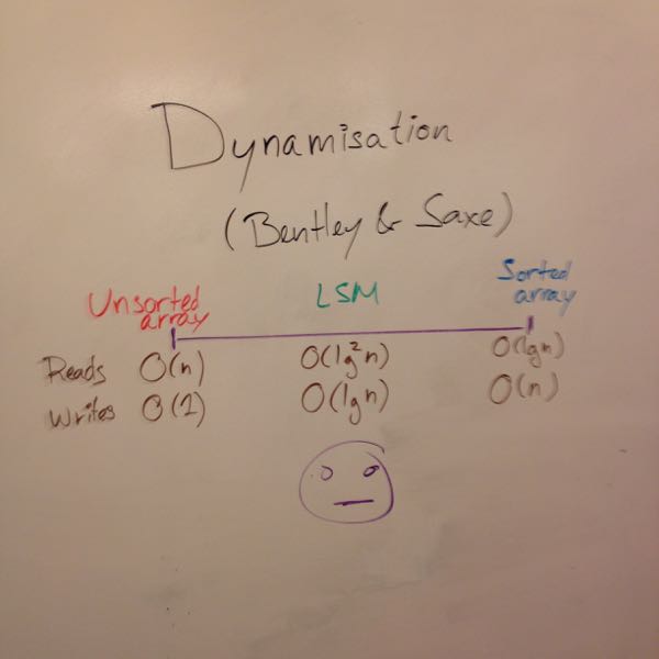
I love searching in sorted arrays, so I kept looking for a way to build simpler search trees on top of that. That lead me to Bentley and Saxe’s (PDF) dynamisation trick. The gist of it is that there’s a family of methods to build dynamic sets on top of static versions. For sorted arrays, one extreme is an unsorted list with fast inserts and slow reads, and the other exactly one sorted array, with slow inserts and fast lookups. The most interesting design point lies in the middle, with \( \log n \) sorted arrays, yielding \( \mathcal{O}(\lg n) \) time inserts and \( \mathcal{O}(\lg\sp{2}n) \) lookups; we can see that design in write-optimised databases. The problem is that my workloads tend to be read heavy.

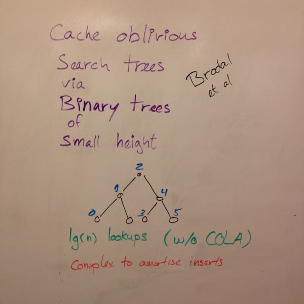
Some time later, I revisited a paper by Brodal, Fagerberg, and Jacob (PDF). They do a lot of clever things to get interesting performance bounds, but I’m really not convinced it’s all worth the complexity¹… especially in the context of our desert island challenge. I did find one trick very interesting: they preserve logarithmic time lookups when binary searching arrays with missing values by recasting these arrays as implicit binary trees and guaranteeing that “NULLs” never have valid entries as descendants. That’s a lot simpler than other arguments based on guaranteeing a minimum density. It’s so much simpler that we can easily make it work with a branch-free binary search: we only need to treat NULLs as \( \pm \infty \) (depending on whether we want a predecessor or a successor).

While lookups are logarithmic time, inserts are \(\mathcal{O}(\lg\sp{2} n) \) time. Still no satisfying answer to the desert island challenge.

I went back to my real research in optimisation, and somehow stumbled on Igal Galperin’s PhD thesis on both on-line optimisation/learning and… simpler balanced binary search trees!

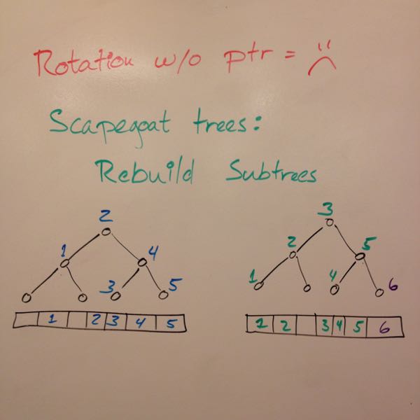
Scapegoat trees (PDF) rebalance by guaranteeing a bound \( \alpha > 0 \) on the relative difference between the optimal depth (\( \lceil\lg n\rceil \)) for a set of \(n\) values and the height (maximal depth) of the balanced tree (at most \( (1+\alpha)\lceil\lg n\rceil \)). The only property that a scapegoat tree has (in addition to those of binary search trees) is this bound on the height of the tree, as a function of its size. Whenever a new node would be inserted at a level too deep for the size of the tree, we go up its ancestors to find a subtree that is small enough to accomodate the newcomer and rebuild it from scratch. I will try to provide an intuition of how they work, but the paper is a much better source.

For a tree of \(n = 14\) elements, we could have \(\alpha = 0.25\), for a maximum depth of \(1.25 \lceil\lg 14\rceil = 5\). Let’s say we attempt to insert a new value, but the tree is structured such that the value would be the child of a leaf that’s already at depth \(5\); we’d violate the (im)balance bound. Instead, we go up until we find an ancestor \(A\) at depth, e.g., \(3\) with \(4\) descendants. The ancestor is shallow enough that it has space for \(5 - 3 = 2\) levels of descendants, for a total height of \(2 + 1 = 3\) for the subtree. A full binary tree of height \(3\) has \(2\sp{3} - 1 = 7\) nodes, and we thus have enough space for \(A\), its \(4\) descendants, and the new node! These 6 values are rebuilt in a near-perfect binary tree: every level must be fully populated, except for the last one.

The criteria to find the scapegoat subtree are a bit annoying to remember–especially given that we don’t want to constantly rebuild the whole tree–but definitely simpler than rotation rules. I feel like that finally solves the desert island balanced search tree challenge… but we still have gapped sorted arrays to address.

What’s interesting about scapegoat trees is that rebalancing is always localised to a subtree. Rotating without explicit pointers is hard (not impossible, amazingly enough), but scapegoat trees just reconstruct the whole subtree, i.e., a contiguous section of the sorted array. That’s easy: slide non-empty values to the right, and redistribute recursively. But, again, finding the scapegoat subtree is annoying.

The \\(\alpha\lg (n)\\) above should read \\((1 + \alpha)\lg n\\), and \\(\lg\lg n + \mathrm{Exp}\cdot\lg n\\) should be \\((\lg\lg n) (1 + \mathrm{Exp})\\).

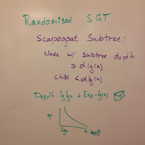
That made me think: what if I randomised scapegoat selection? Rather than counting elements in subtrees, I could approximate that probabilistically by sampling from an exponential distribution… which we can easily approximate with the geometric for \(p = 0.5\) by counting leading zeros in bitstrings.

I’m still not totally convinced that it works, but I vaguely remember successfully testing an implementation and sketching a proof that we can find the scapegoat subtree by going up according to a scaled geometric to preserve amortised logarithmic time inserts. The probability function decreases quickly enough that we preserve logarithmic time inserts on average, yet slowly enough that we can expect to redistribute a region before it runs out of space.

The argument is convoluted, but the general idea is based on the observation that, in a tree of maximum height \(m\), a subtree at depth \(k\) can contain at most \(n\sp\prime = 2\sp{m - k + 1} - 1\) elements (including the subtree’s root).

We only violate the imbalance bound in a subtree if we attempt to insert more than \(n\sp\prime\) elements in it. Rebalancing works by designating the shallowest subtree that’s not yet full as the scapegoat. We could simplify the selection of the scapegoat tree by counting the number of inserts in each subtree, but that’d waste a lot of space. Instead, we count probabilistically and ensure that there’s a high probability (that’s why we always go up by at least \(\lg \lg n\) levels) that each subtree will be rebalanced at least once before it hits its insertion count limit. The memoryless property of the geometric distribution means that this works even after a rebalance. If we eventually fail to find space, it’s time to completely rebuild the subtree; this case happens rarely enough (\(p \approx \frac{\lg n}{n}\)) that the amortised time for insertions is still logarithmic.

Again \\(2\sp{\alpha \lg n}\\) should be \\(2\sp{(1 + \alpha)\lg n}\\).

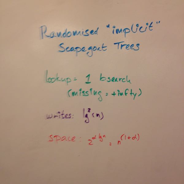
We can do the same thing when embedding scapegoat trees in implicit trees. The problem is that a multiplicative overhead in depth results in an exponential space blowup. The upside is that the overhead is tunable: we can use less space at the expense of slowing down inserts.

In fact, if we let \( \alpha \rightarrow 0 \), we find Brodal et al’s scheme (I don’t know why they didn’t just cite Galperin and Rivest on scapegoat trees)! The difference is that we are now pretty sure that we can easily let a random number generator guide our redistribution.

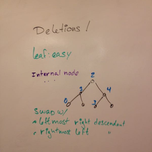
I only covered insertions and lookups so far. It turns out that deletions in scapegoat trees are easy: replace the deleted node with one of its leaves. Deletions should also eventually trigger a full rebalance to guarantee logarithmic time lookups.

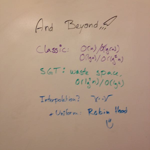
Classical implicit representations for sorted sets make us choose between appallingly slow (linear time) inserts and slow lookups. With stochastic scapegoat trees embedded in implicit binary trees, we get logarithmic time lookups, and we have a continuum of choices between wasting an exponential amount of space and slow \( \mathcal{O}(\lg\sp{2} n) \) inserts. In order to get there, we had to break one rule: we allowed ourselves \(\mathcal{O}(n)\) additional space, rather than \(\mathcal{o}(n)\), but it’s all empty space.

What other rule or assumption can we challenge (while staying true to the spirit of searching in arrays)?

I’ve been thinking about interpolation lately: what if we had a monotone (not necessarily injective) function to map from the set’s domain to machine integers? That’d let us bucket values or interpolate to skip the first iterations of the search. If we can also assume that the keys are uniformly distributed once mapped to integers, we can use a linear Robin Hood hash table: with a linear (but small) space overhead, we get constant time expected inserts and lookups, and what seems to be \( O(\lg \lg n) \) worst case² lookups with high probability.

Something else is bothering me. We embed in full binary trees, and thus binary search over arrays of size \(2\sp{n} - 1\)… and we know that’s a bad idea. We could switch to ternary trees, but that means inserts and deletes must round to the next power of three. Regular div-by-mul and scaling back up by the divisor always works; is there a simpler way to round to a power of three or to find the remainder by such a number?

I don’t know! Can anyone offer insights or suggest new paths to explore?

---