This post goes over some code that I pushed to github today. All the snippets below should be in the repo, which also includes C and Python code with the same structure.

I recently resumed thinking about balls and bins for hash tables. This time, I’m looking at large bins (on the order of one 2MB huge page). There are many hashing methods with solid worst-case guarantees that unfortunately query multiple uncorrelated locations; I feel like we could automatically adapt them to modern hierarchical storage (or address translation) to make them more efficient, for a small loss in density.

In theory, large enough bins can be allocated statically with a minimal waste of space. I wanted some actual non-asymptotic numbers, so I ran numerical experiments and got the following distribution of global utilisation (fill rate) when the first bin fills up.

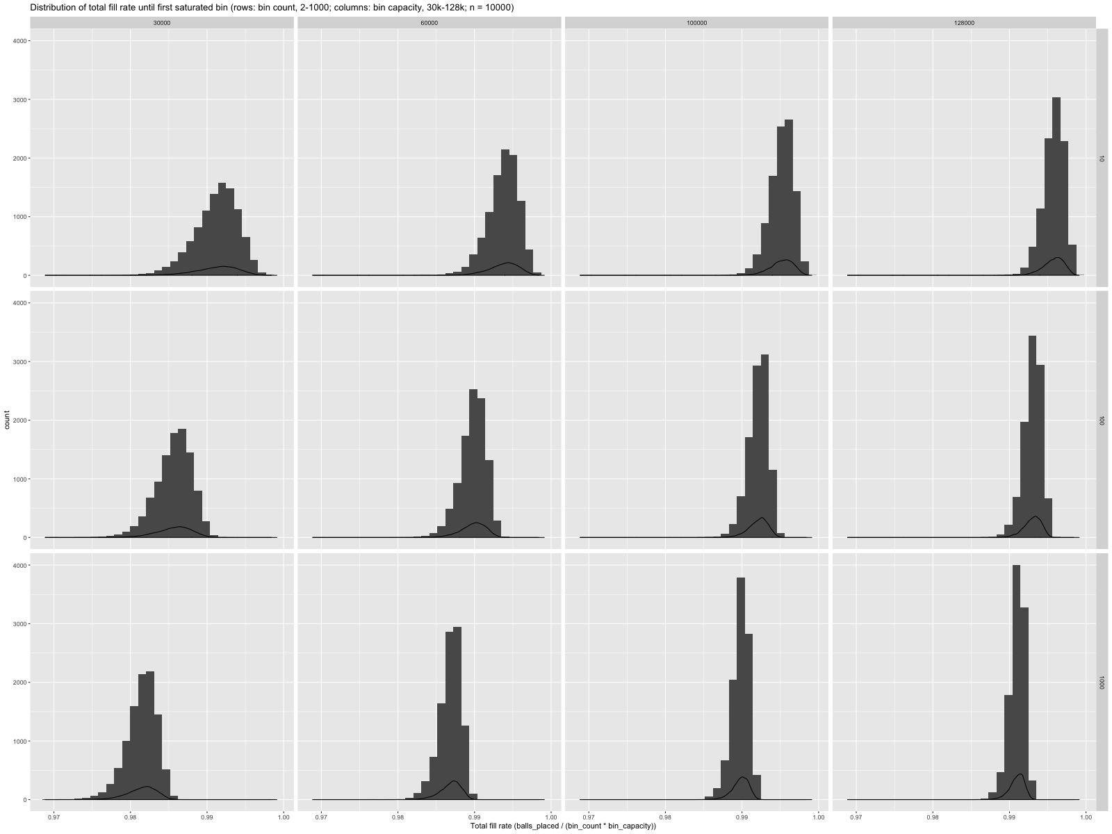
It looks like, even with one thousand bins of thirty thousand values, we can expect almost 98% space utilisation until the first bin saturates. I want something more formal.

Could I establish something like a service level objective, “When distributing balls randomly between one thousand bins with individual capacity of thirty thousand balls, we can utilise at least 98% of the total space before a bin fills up, x% of the time?”

The natural way to compute the “x%” that makes the proposition true is to first fit a distribution on the observed data, then find out the probability mass for that distribution that lies above 98% fill rate. Fitting distributions takes a lot of judgment, and I’m not sure I trust myself that much.

Alternatively, we can observe independent identically distributed fill rates, check if they achieve 98% space utilisation, and bound the success rate for this Bernoulli process.

There are some non-trivial questions associated with this approach.

How do we know when to stop generating more observations… without fooling ourselves with $p$-hacking?
How can we generate something like a confidence interval for the success rate?

Thankfully, I have been sitting on a software package to compute satisfaction rate for exactly this kind of SLO-type properties, properties of the form “this indicator satisfies $PREDICATE x% of the time,” with arbitrarily bounded false positive rates.

The code takes care of adaptive stopping, generates a credible interval, and spits out a report like this : we see the threshold (0.98), the empirical success rate estimate (0.993 ≫ 0.98), a credible interval for the success rate, and the shape of the probability mass for success rates.

This post shows how to compute credible intervals for the Bernoulli’s success rate, how to implement a dynamic stopping criterion, and how to combine the two while compensating for multiple hypothesis testing. It also gives two examples of converting more general questions to SLO form, and answers them with the same code.

Credible intervals for the Binomial

If we run the same experiment $n$ times, and observe $a$ successes ($b = n - a$ failures), it’s natural to ask for an estimate of the success rate $p$ for the underlying Bernoulli process, assuming the observations are independent and identically distributed.

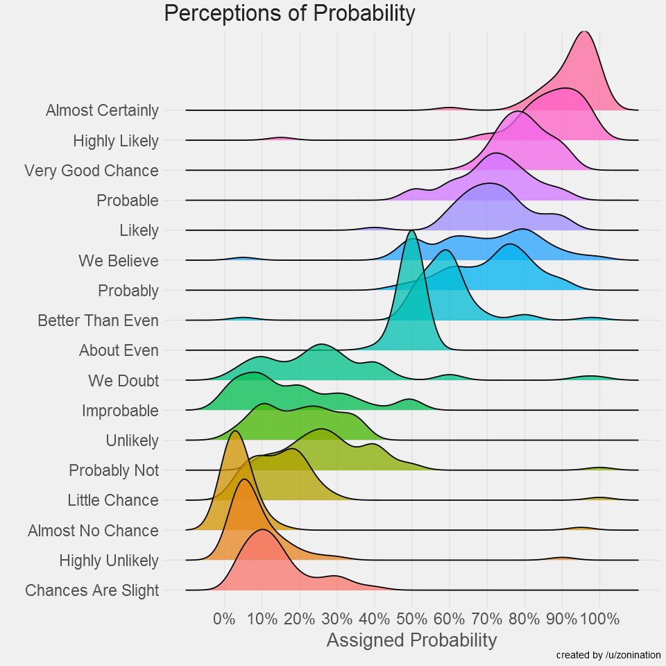
Intuitively, that estimate should be close to $a / n$, the empirical success rate, but that’s not enough. I also want something that reflects the uncertainty associated with small $n$, much like in the following ridge line plot, where different phrases are assigned not only a different average probability, but also a different spread.

I’m looking for an interval of plausible success rates $p$ that responds to both the empirical success rate $a / n$ and the sample size $n$; that interval should be centered around $a / n$, be wide when $n$ is small, and become gradually tighter as $n$ increases.

The Bayesian approach is straightforward, if we’re willing to shut up and calculate. Once we fix the underlying success rate $p = \hat{p}$, the conditional probability of observing $a$ successes and $b$ failures is

\[P((a, b) | p = \hat{p}) \sim \hat{p}^{a} \cdot (1 - \hat{p})^{b},\] where the right-hand side is a proportion¹, rather than a probability.

We can now apply Bayes’s theorem to invert the condition and the event. The inversion will give us the conditional probability that $p = \hat{p}$, given that we observed $a$ successes and $b$ successes. We only need to impose a prior distribution on the underlying rate $p$. For simplicity, I’ll go with the uniform $U[0, 1]$, i.e., every success rate is equally plausible, at first. We find

\[P(p = \hat{p} | (a, b)) = \frac{P((a, b) | p = \hat{p}) P(p = \hat{p})}{P(a, b)}.\]

We already picked the uniform prior, $P(p = \hat{p}) = 1,\quad\forall\, \hat{p}\in [0,1],$ and the denominator is a constant with respect to $\hat{p}$. The expression simplifies to

\[P(p = \hat{p} | (a, b)) \sim \hat{p}\sp{a} \cdot (1 - \hat{p})\sp{b},\] or, if we normalise to obtain a probability,

\[P(p = \hat{p} | (a, b)) = \frac{\hat{p}\sp{a} \cdot (1 - \hat{p})\sp{b}}{\int\sb{0}\sp{1} \hat{p}\sp{a} \cdot (1 - \hat{p})\sp{b}\, d\hat{p}} = \textrm{Beta}(a+1, b+1).\]

A bit of calculation, and we find that our credibility estimate for the underlying success rate follows a Beta distribution. If one is really into statistics, they can observe that the uniform prior distribution is just the $\textrm{Beta}(1, 1)$ distribution, and rederive that the Beta is the conjugate distribution for the Binomial distribution.

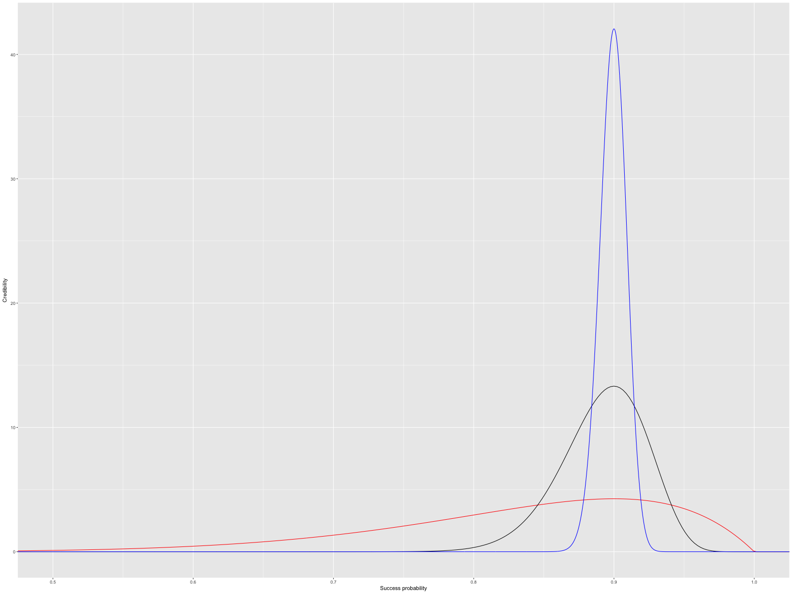
For me, it suffices to observe that the distribution $\textrm{Beta}(a+1, b+1)$ is unimodal, does peak around $a / (a + b)$, and becomes tighter as the number of observations grows. In the following image, I plotted three Beta distributions, all with empirical success rate 0.9; red corresponds to $n = 10$ ($a = 9$, $b = 1$, $\textrm{Beta}(10, 2)$), black to $n = 100$ ($\textrm{Beta}(91, 11)$), and blue to $n = 1000$ ($\textrm{Beta}(901, 101)$).

We calculated, and we got something that matches my intuition. Before trying to understand what it means, let’s take a detour to simply plot points from that un-normalised proportion function $\hat{p}\sp{a} \cdot (1 - \hat{p})\sp{b}$, on an arbitrary $y$ axis.

Let $\hat{p} = 0.4$, $a = 901$, $b = 101$. Naïvely entering the expression at the REPL yields nothing useful.

CL-USER> (* (expt 0.4d0 901) (expt (- 1 0.4d0) 101))
0.0d0

The issue here is that the un-normalised proportion is so small that it underflows double floats and becomes a round zero. We can guess that the normalisation factor $\frac{1}{\mathrm{Beta}(\cdot,\cdot)}$ quickly grows very large, which will bring its own set of issues when we do care about the normalised probability.

How can we renormalise a set of points without underflow? The usual trick to handle extremely small or large magnitudes is to work in the log domain. Rather than computing $\hat{p}\sp{a} \cdot (1 - \hat{p})\sp{b}$, we shall compute

\[\log\left[\hat{p}\sp{a} \cdot (1 - \hat{p})\sp{b}\right] = a \log\hat{p} + b \log (1 - \hat{p}).\]

CL-USER> (+ (* 901 (log 0.4d0)) (* 101 (log (- 1 0.4d0))))
-877.1713374189787d0
CL-USER> (exp *)
0.0d0

That’s somewhat better: the log-domain value is not $-\infty$, but converting it back to a regular value still gives us 0.

The $\log$ function is monotonic, so we can find the maximum proportion value for a set of points, and divide everything by that maximum value to get plottable points. There’s one last thing that should change: when $x$ is small, $1 - x$ will round most of $x$ away. Instead of (log (- 1 x)), we should use (log1p (- x)) to compute $\log (1 + -x) = \log (1 - x)$. Common Lisp did not standardise log1p, but SBCL does have it in internals, as a wrapper around libm. We’ll just abuse that for now.

CL-USER> (defun proportion (x) (+ (* 901 (log x)) (* 101 (sb-kernel:%log1p (- x)))))
PROPORTION
CL-USER> (defparameter *points* (loop for i from 1 upto 19 collect (/ i 20d0)))
*POINTS*
CL-USER> (reduce #'max *points* :key #'proportion)
-327.4909190001001d0

We have to normalise in the log domain, which is simply a subtraction: $\log(x / y) = \log x - \log y$. In the case above, we will subtract $-327.49\ldots$, or add a massive $327.49\ldots$ to each log proportion (i.e., multiply by $10\sp{142}$). The resulting values should have a reasonably non-zero range.

CL-USER> (mapcar (lambda (x) (cons x (exp (- (proportion x) *)))) *points*)
((0.05d0 . 0.0d0)
 (0.1d0 . 0.0d0)
 [...]
 (0.35d0 . 3.443943164733533d-288)
 [...]
 (0.8d0 . 2.0682681158181894d-16) 
 (0.85d0 . 2.6252352579425913d-5)
 (0.9d0 . 1.0d0)
 (0.95d0 . 5.65506756824607d-10))

There’s finally some signal in there. This is still just an un-normalised proportion function, not a probability density function, but that’s already useful to show the general shape of the density function, something like the following, for $\mathrm{Beta}(901, 101)$.

Finally, we have a probability density function for the Bayesian update of our belief about the success rate after $n$ observations of a Bernoulli process, and we know how to compute its proportion function. Until now, I’ve carefully avoided the question of what all these computations even mean. No more (:

The Bayesian view assumes that the underlying success rate (the value we’re trying to estimate) is unknown, but sampled from some distribution. In our case, we assumed a uniform distribution, i.e., that every success rate is a priori equally likely. We then observe $n$ outcomes (successes or failures), and assign an updated probability to each success rate. It’s like a many-world interpretation in which we assume we live in one of a set of worlds, each with a success rate sampled from the uniform distribution; after observing 900 successes and 100 failures, we’re more likely to be in a world where the success rate is 0.9 than in one where it’s 0.2. With Bayes’s theorem to formalise the update, we assign posterior probabilities to each potential success rate value.

We can compute an equal-tailed credible interval from that $\mathrm{Beta}(a+1,b+1)$ posterior distribution by excluding the left-most values, $[0, l)$, such that the Beta CDF (cumulative distribution function) at $l$ is $\varepsilon / 2$, and doing the same with the right most values to cut away $\varepsilon / 2$ of the probability density. The CDF for $\mathrm{Beta}(a+1,b+1)$ at $x$ is the incomplete beta function, $I\sb{x}(a+1,b+1)$. That function is really hard to compute (this technical report detailing Algorithm 708 deploys five different evaluation strategies), so I’ll address that later.

The more orthodox “frequentist” approach to confidence intervals treats the whole experiment, from data colleaction to analysis (to publication, independent of the observations 😉) as an Atlantic City algorithm: if we allow a false positive rate of $\varepsilon$ (e.g., $\varepsilon=5\%$), the experiment must return a confidence interval that includes the actual success rate (population statistic or parameter, in general) with probability $1 - \varepsilon$, for any actual success rate (or underlying population statistic / parameter). When the procedure fails, with probability at most $\varepsilon$, it is allowed to fail in an arbitrary manner.

The same Atlantic City logic applies to $p$-values. An experiment (data collection and analysis) that accepts when the $p$-value is at most $0.05$ is an Atlantic City algorithm that returns a correct result (including “don’t know”) with probability at least $0.95$, and is otherwise allowed to yield any result with probability at most $0.05$. The $p$-value associated with a conclusion, e.g., “success rate is more than 0.8” (the confidence level associated with an interval) means something like “I’m pretty sure that the success rate is more than 0.8, because the odds of observing our data if that were false are small (less than 0.05).” If we set that threshold (of 0.05, in the example) ahead of time, we get an Atlantic City algorithm to determine if “the success rate is more than 0.8” with failure probability 0.05. (In practice, reporting is censored in all sorts of ways, so…)

There are ways to recover a classical confidence interval, given $n$ observations from a Bernoulli. However, they’re pretty convoluted, and, as Jaynes argues in his note on confidence intervals, the classical approach gives values that are roughly the same² as the Bayesian approach… so I’ll just use the Bayesian credibility interval instead.

See this stackexchange post for a lot more details.

Dynamic stopping for Binomial testing

The way statistics are usually deployed is that someone collects a data set, as rich as is practical, and squeezes that static data set dry for significant results. That’s exactly the setting for the credible interval computation I sketched in the previous section.

When studying the properties of computer programs or systems, we can usually generate additional data on demand, given more time. The problem is knowing when it’s ok to stop wasting computer time, because we have enough data… and how to determine that without running into multiple hypothesis testing issues (ask anyone who’s run A/B tests).

Here’s an example of an intuitive but completely broken dynamic stopping criterion. Let’s say we’re trying to find out if the success rate is less than or greater than 90%, and are willing to be wrong 5% of the time. We could get $k$ data points, run a statistical test on those data points, and stop if the data let us conclude with 95% confidence that the underlying success rate differs from 90%. Otherwise, collect $2k$ fresh points, run the same test; collect $4k, \ldots, 2\sp{i}k$ points. Eventually, we’ll have enough data.

The issue is that each time we execute the statistical test that determines if we should stop, we run a 5% risk of being totally wrong. For an extreme example, if the success rate is exactly 90%, we will eventually stop, with probability 1. When we do stop, we’ll inevitably conclude that the success rate differs from 90%, and we will be wrong. The worst-case (over all underlying success rates) false positive rate is 100%, not 5%!

In my experience, programmers tend to sidestep the question by wasting CPU time with a large, fixed, number of iterations… people are then less likely to run our statistical tests, since they’re so slow, and everyone loses (the other popular option is to impose a reasonable CPU budget, with error thresholds so lax we end up with a smoke test).

Robbins, in Statistical Methods Related to the Law of the Iterated Logarithm, introduces a criterion that, given a threshold success rate $p$ and a sequence of (infinitely many!) observations from the same Bernoulli with unknown success rate parameter, will be satisfied infinitely often when $p$ differs from the Bernoulli’s success rate. Crucially, Robbins also bounds the false positive rate, the probability that the criterion be satisfied even once in the infinite sequence of observations if the Bernoulli’s unknown success rate is exactly equal to $p$. That criterion is

\[{n \choose a} p\sp{a} (1-p)\sp{n-a} \leq \frac{\varepsilon}{n+1},\]

where $n$ is the number of observations, $a$ the number of successes, $p$ the threshold success rate, and $\varepsilon$ the error (false positive) rate. As the number of observation grows, the criterion becomes more and more stringent to maintain a bounded false positive rate over the whole infinite sequence of observations.

There are similar “Confidence Sequence” results for other distributions (see, for example, this paper of Lai), but we only care about the Binomial here.

More recently, Ding, Gandy, and Hahn showed that Robbins’s criterion also guarantees that, when it is satisfied, the empirical success rate ($a/n$) lies on the correct side of the threshold $p$ (same side as the actual unknown success rate) with probability $1-\varepsilon$. This result leads them to propose the use of Robbins’s criterion to stop Monte Carlo statistical tests, which they refer to as the Confidence Sequence Method (CSM).

(defun csm-stop-p (successes failures threshold eps)
  "Pseudocode, this will not work on a real machine."
  (let ((n (+ successes failures)))
    (<= (* (choose n successes) 
           (expt threshold successes)
           (expt (- 1 threshold) failures))
        (/ eps (1+ n)))))

We may call this predicate at any time with more independent and identically distributed results, and stop as soon as it returns true.

The CSM is simple (it’s all in Robbins’s criterion), but still provides good guarantees. The downside is that it is conservative when we have a limit on the number of observations: the method “hedges” against the possibility of having a false positive in the infinite number of observations after the limit, observations we will never make. For computer-generated data sets, I think having a principled limit is pretty good; it’s not ideal to ask for more data than strictly necessary, but not a blocker either.

In practice, there are still real obstacles to implementing the CSM on computers with finite precision (floating point) arithmetic, especially since I want to preserve the method’s theoretical guarantees (i.e., make sure rounding is one-sided to overestimate the left-hand side of the inequality).

If we implement the expression well, the effect of rounding on correctness should be less than marginal. However, I don’t want to be stuck wondering if my bad results are due to known approximation errors in the method, rather than errors in the code. Moreover, if we do have a tight expression with little rounding errors, adjusting it to make the errors one-sided should have almost no impact. That seems like a good trade-off to me, especially if I’m going to use the CSM semi-automatically, in continuous integration scripts, for example.

One look at csm-stop-p shows we’ll have the same problem we had with the proportion function for the Beta distribution: we’re multiplying very small and very large values. We’ll apply the same fix: work in the log domain and exploit $\log$’s monotonicity.

\[{n \choose a} p\sp{a} (1-p)\sp{n-a} \leq \frac{\varepsilon}{n+1}\]

becomes

\[\log {n \choose a} + a \log p + (n-a)\log (1-p) \leq \log\varepsilon -\log(n+1),\] or, after some more expansions, and with $b = n - a$,

\[\log n! - \log a! - \log b! + a \log p + b \log(1 - p) + \log(n+1) \leq \log\varepsilon.\]

The new obstacle is computing the factorial $x!$, or the log-factorial $\log x!$. We shouldn’t compute the factorial iteratively: otherwise, we could spend more time in the stopping criterion than in the data generation subroutine. Robbins has another useful result for us:

\[\sqrt{2\pi} n\sp{n + 1/2} \exp(-n) \exp\left(\frac{1}{12n+1}\right) < n! < \sqrt{2\pi} n\sp{n + 1/2} \exp(-n) \exp\left(\frac{1}{12n}\right),\]

or, in the log domain,

\[\log\sqrt{2\pi} + \left(n + \frac{1}{2}\right)\log n -n + \frac{1}{12n+1} < \log n! < \log\sqrt{2\pi} + \left(n + \frac{1}{2}\right)\log n -n +\frac{1}{12n}.\]

This double inequality gives us a way to over-approximate $\log {n \choose a} = \log \frac{n!}{a! b!} = \log n! - \log a! - \log b!,$ where $b = n - a$:

\[\log {n \choose a} < -\log\sqrt{2\pi} + \left(n + \frac{1}{2}\right)\log n -n +\frac{1}{12n} - \left(a + \frac{1}{2}\right)\log a +a - \frac{1}{12a+1} - \left(b + \frac{1}{2}\right)\log b +b - \frac{1}{12b+1},\]

where the right-most expression in Robbins’s double inequality replaces $\log n!$, which must be over-approximated, and the left-most $\log a!$ and $\log b!$, which must be under-approximated.

Robbins’s approximation works well for us because, it is one-sided, and guarantees that the (relative) error in $n!$, $\frac{\exp\left(\frac{1}{12n}\right) - \exp\left(\frac{1}{12n+1}\right)}{n!},$ is small, even for small values like $n = 5$ (error $< 0.0023\%$), and decreases with $n$: as we perform more trials, the approximation is increasingly accurate, thus less likely to spuriously prevent us from stopping.

Now that we have a conservative approximation of Robbins’s criterion that only needs the four arithmetic operations and logarithms (and log1p), we can implement it on a real computer. The only challenge left is regular floating point arithmetic stuff: if rounding must occur, we must make sure it is in a safe (conservative) direction for our predicate.

Hardware usually lets us manipulate the rounding mode to force floating point arithmetic operations to round up or down, instead of the usual round to even. However, that tends to be slow, so most language (implementations) don’t support changing the rounding mode, or do so badly… which leaves us in a multi-decade hardware/software co-evolution Catch-22.

I could think hard and derive tight bounds on the round-off error, but I’d rather apply a bit of brute force. IEEE-754 compliant implementations must round the four basic operations correctly. This means that $z = x \oplus y$ is at most half a ULP away from $x + y,$ and thus either $z = x \oplus y \geq x + y,$ or the next floating point value after $z,$ $z^\prime \geq x + y$. We can find this “next value” portably in Common Lisp, with decode-float/scale-float, and some hand-waving for denormals.

(defun next (x &optional (delta 1))
  "Increment x by delta ULPs. Very conservative for
   small (0/denormalised) values."
  (declare (type double-float x)
           (type unsigned-byte delta))
  (let* ((exponent (nth-value 1 (decode-float x)))
         (ulp (max (scale-float double-float-epsilon exponent)
                   least-positive-normalized-double-float)))
    (+ x (* delta ulp))))

I prefer to manipulate IEEE-754 bits directly. That’s theoretically not portable, but the platforms I care about make sure we can treat floats as sign-magnitude integers.

#+sbcl
(progn
  (declaim (inline %float-bits %bits-float next prev))
  (defun %float-bits (x)
    "Convert a double float x to sign-extended sign/magnitude, and
     then to 2's complement."
    (declare (type double-float x))
    (let* ((hi (sb-kernel:double-float-high-bits x))
           (lo (sb-kernel:double-float-low-bits x))
           (word (+ (ash (ldb (byte 31 0) hi) 32) lo)))
      ;; hi is the high half of the 64 bit sign-magnitude
      ;; representation… in two's complement. Extract the significand,
      ;; and then apply the sign bit. We want to preserve signed zeros,
      ;; so return -1 - word instead of -word.
      ;;
      ;; (- -1 word) = (lognot word) = (logxor word -1).
      (logxor word (ash hi -32))))

  (defun %bits-float (bits)
    "Convert 2's complement to sign-extended sign/magnitude, then
     double float."
    (declare (type (signed-byte 64) bits))
    ;; convert back to sign-magnitude: if bits is negative, all but the
    ;; sign bit must be flipped again.
    (let ((bits (logxor bits
                        (ldb (byte 63 0) (ash bits -64)))))
      (sb-kernel:make-double-float (ash bits -32)
                                   (ldb (byte 32 0) bits))))

  (defun next (x &optional (delta 1))
    "Increment x by delta ULPs."
    (declare (type double-float x)
             (type unsigned-byte delta))
    (%bits-float (+ (%float-bits x) delta)))

  (defun prev (x &optional (delta 1))
    "Decrement x by delta ULPs."
    (declare (type double-float x)
             (type unsigned-byte delta))
    (%bits-float (- (%float-bits x) delta))))

CL-USER> (double-float-bits pi)
4614256656552045848
CL-USER> (double-float-bits (- pi))
-4614256656552045849

The two’s complement value for pi is one less than (- (double-float-bits pi)) because two’s complement does not support signed zeros.

CL-USER> (eql 0 (- 0))
T
CL-USER> (eql 0d0 (- 0d0))
NIL
CL-USER> (double-float-bits 0d0)
0
CL-USER> (double-float-bits -0d0)
-1

We can quickly check that the round trip from float to integer and back is an identity.

CL-USER> (eql pi (bits-double-float (double-float-bits pi)))
T
CL-USER> (eql (- pi) (bits-double-float (double-float-bits (- pi))))
T
CL-USER> (eql 0d0 (bits-double-float (double-float-bits 0d0)))
T
CL-USER> (eql -0d0 (bits-double-float (double-float-bits -0d0)))
T

We can also check that incrementing or decrementing the integer representation does increase or decrease the floating point value.

CL-USER> (< (bits-double-float (1- (double-float-bits pi))) pi)
T
CL-USER> (< (bits-double-float (1- (double-float-bits (- pi)))) (- pi))
T
CL-USER> (bits-double-float (1- (double-float-bits 0d0)))
-0.0d0
CL-USER> (bits-double-float (1+ (double-float-bits -0d0)))
0.0d0
CL-USER> (bits-double-float (1+ (double-float-bits 0d0)))
4.9406564584124654d-324
CL-USER> (bits-double-float (1- (double-float-bits -0d0)))
-4.9406564584124654d-324

The code doesn’t handle special values like infinities or NaNs, but that’s out of scope for the CSM criterion anyway. That’s all we need to nudge the result of the four operations to guarantee an over- or under- approximation of the real value. We can also look at the documentation for our libm (e.g., for GNU libm) to find error bounds on functions like log; GNU claims their log is never off by more than 3 ULP. We can round up to the fourth next floating point value to obtain a conservative upper bound on $\log x$.

log

(declaim (type (unsigned-byte 31) *libm-error-limit*))
(defvar *libm-error-limit* 4
  "Assume libm is off by less than 4 ULPs.")

(declaim (inline log-up log-down))
(defun log-up (x)
  "Conservative upper bound on log(x)."
  (declare (type double-float x))
  (next (log x) *libm-error-limit*))

(defun log-down (x)
  "Conservative lower bound on log(x)."
  (declare (type double-float x))
  (prev (log x) *libm-error-limit*))

#+sbcl
(progn
  (declaim (inline log1p-up log1p-down))
  (defun log1p-up (x)
    "Convervative upper bound on log(1 + x)."
    (declare (type double-float x))
    (next (sb-kernel:%log1p x) *libm-error-limit*))

  (defun log1p-down (x)
    "Conservative lower bound on log(1 + x)"
    (declare (type double-float x))
    (prev (sb-kernel:%log1p x) *libm-error-limit*)))

I could go ahead and use the building blocks above (ULP nudging for directed rounding) to directly implement Robbins’s criterion,

\[\log {n \choose a} + a \log p + b\log (1-p) + \log(n+1) \leq \log\varepsilon,\]

with Robbins’s factorial approximation,

However, even in the log domain, there’s a lot of cancellation: we’re taking the difference of relatively large numbers to find a small result. It’s possible to avoid that by re-associating some of the terms above, e.g., for $a$:

\[-\left(a + \frac{1}{2}\right) \log a + a - a \log p = -\frac{\log a}{2} + a (-\log a + 1 - \log p).\]

Instead, I’ll just brute force things (again) with Kahan summation. Shewchuk’s presentation in Adaptive Precision Floating-Point Arithmetic and Fast Robust Geometric Predicates highlights how the only step where we may lose precision to rounding is when we add the current compensation term to the new summand. We can implement Kahan summation with directed rounding in only that one place: all the other operations are exact!

"kahan summation"

;;; Kahan-style summation.
;;;
;;; Represent the accumulator as an evaluated sum of two doubles. As
;;; long as the compensation term is initially 0, the result is a safe
;;; upper bound on the real value, and the two terms are
;;; "non-overlapping."  For more details, see "Adaptive Precision
;;; Floating-Point Arithmetic and Fast Robust Geometric Predicates",
;;; Shewchuk, 1997; Technical report CMU-CS-96-140R / Discrete & Comp
;;; Geom 18(3), October 1997. Theorem 6 in particular.

(declaim (inline sum-update-up sum-update-finish))
(defun sum-update-up (accumulator compensation term &optional ordered)
  "Given an evaluated sum
     (accumulator + compensation),
   return a new unevaluated sum for an upper bound on
     (accumulator + compensation + term).

   If ordered, assume
     term < accumulator,
   or
     accumulator = compensation = 0."
  (declare (type double-float accumulator compensation
                 term))
  (when (and (not ordered)
             (< (abs accumulator) (abs term)))
    (rotatef accumulator term))
  (let* ((rest-1 (next (+ compensation term))) ; safe upper bound on c + t
         (rest (if (<= compensation 0d0)       ; tighter, still safe.
                   (min term rest-1)
                   rest-1))
         ;; Perform a Dekker sum of accumulator + rest. The result is
         ;; exact, so no need for next/prev here.
         ;;
         ;; Precondition: |accumulator| >= |rest| (or accumulator = 0).
         (a accumulator)
         (b rest)
         (x (+ a b))
         (b-virtual (- x a))     ; b-virtual = value really added to a
         (y (- b b-virtual)))
    (values x y)))

(defun sum-update-finish (accumulator compensation)
  "Return a conservative upper bound for accumulator + compensation.

   In theory, (+ accumulator compensation) is equal to accumulator.
   In practice, it doesn't hurt to do this right. The second return
   value is the new compensation term (should never be positive)."
  (declare (type double-float accumulator compensation))
  (let* ((raw-sum (next (+ accumulator compensation)))
         (sum (if (> compensation 0d0)
                  raw-sum
                  ;; if compensation <= 0, acc is already an upper
                  ;; bound.
                  (min accumulator raw-sum)))
         (delta (- sum accumulator)))
    (assert (>= delta compensation))
    (values sum (- compensation delta))))

(declaim (ftype (function (&rest double-float)
                          (values double-float double-float &optional))
                sum-up))
(defun sum-up (&rest values)
  "Conservative upper bound for the sum of values, with a Kahan
   summation loop."
  (let ((acc 0d0)
        (err 0d0))
    (dolist (value values (sum-update-finish acc err))
      (setf (values acc err)
            (sum-update-up acc err value)))))

We need one last thing to implement $\log {n \choose a}$, and then Robbins’s confidence sequence: a safely rounded floating-point value approximation of $-\log \sqrt{2 \pi}$. I precomputed one with computable-reals:

CL-USER> (computable-reals:-r
          (computable-reals:log-r
           (computable-reals:sqrt-r computable-reals:+2pi-r+)))
-0.91893853320467274178...
CL-USER> (computable-reals:ceiling-r 
          (computable-reals:*r *
                               (ash 1 53)))
-8277062471433908
-0.65067431749790398594...
CL-USER> (* -8277062471433908 (expt 2d0 -53))
-0.9189385332046727d0
CL-USER> (computable-reals:-r (rational *)
                              ***)
+0.00000000000000007224...

We can safely replace $-\log\sqrt{2\pi}$ with -0.9189385332046727d0, or, equivalently, (scale-float -8277062471433908.0d0 -53), for an upper bound. If we wanted a lower bound, we could decrement the integer significand by one.

log-choose

;;; Upper bound for log c(n, s).

(declaim (type double-float *minus-log-sqrt-2pi*))
(defvar *minus-log-sqrt-2pi* -0.9189385332046727d0
  "Smallest double precision value > -log sqrt(2pi).")

(declaim (ftype (function ((unsigned-byte 49) (unsigned-byte 49))
                          (values double-float double-float &optional))
                robbins-log-choose))
(defun robbins-log-choose (n s)
  "Compute a conservative upper bound on log c(n, s) based on
   Robbins's bounds for k!."
  (check-type n (unsigned-byte 49)) ;; ensure 53 bit arith is exact.
  (check-type s (unsigned-byte 49))
  (assert (<= 0 s n))
  ;; Handle easy cases, where c(n, s) is 1 or n.
  (when (or (= n s)
            (zerop s))
    (return-from robbins-log-choose (values 0d0 0d0)))
  (when (or (= s 1)
            (= s (1- n)))
    (return-from robbins-log-choose (values (log-up (float n 1d0))
                                            0d0)))
  (let* ((n (float n 1d0))
         (s (float s 1d0))
         (n-s (float (- n s) 1d0))
         (l1 (next (* (+ n .5d0) (log-up n)))) ; (+ n .5d0) is exact.
         (l2 (next (- (* (+ s .5d0) (log-down s)))))
         (l3 (next (- (* (+ n-s .5d0) (log-down n-s)))))
         (r1 (next (/ (* 12d0 n))))          ; (* 12d0 n) is exact.
         (r2 (next (- (/ (1+ (* 12d0 s)))))) ; also exact.
         (r3 (next (- (/ (1+ (* 12d0 n-s)))))))
    (sum-up *minus-log-sqrt-2pi*
            l1 l2 l3
            r1 r2 r3)))

We can quickly check against an exact implementation with computable-reals and a brute force factorial.

CL-USER> (defun cr-log-choose (n s)
           (computable-reals:-r
            (computable-reals:log-r (alexandria:factorial n))
            (computable-reals:log-r (alexandria:factorial s))
            (computable-reals:log-r (alexandria:factorial (- n s)))))
CR-LOG-CHOOSE
CL-USER> (computable-reals:-r (rational (robbins-log-choose 10 5))
                              (cr-log-choose 10 5))
+0.00050526703375914436...
CL-USER> (computable-reals:-r (rational (robbins-log-choose 1000 500))
                              (cr-log-choose 1000 500))
+0.00000005551513197557...
CL-USER> (computable-reals:-r (rational (robbins-log-choose 1000 5))
                              (cr-log-choose 1000 5))
+0.00025125559085509706...

That’s not obviously broken: the error is pretty small, and always positive.

Given a function to over-approximate log-choose, the Confidence Sequence Method’s stopping criterion is straightforward.

csm

(declaim (ftype (function ((unsigned-byte 49)
                           (real (0) (1))
                           (unsigned-byte 49)
                           real)
                          (values boolean double-float &optional))
                csm))
(defun csm (n alpha s log-eps)
  "Given n trials and s sucesses, are we reasonably sure that the
  success rate is *not* alpha (with a false positive rate < exp(log-eps))?

  Answer that question with Ding, Gandy, and Hahn's confidence
  sequence method (CSM). The second return value is an estimate of the
  false positive target rate we would need to stop here. This value
  should only be used for reporting; the target rate eps should always
  be fixed before starting the experiment."
  (check-type n (unsigned-byte 49))
  (check-type alpha (real (0) (1)))
  (check-type s (unsigned-byte 49))
  (check-type log-eps real)
  (assert (<= 0 s n))
  (let* ((log-choose (robbins-log-choose n s))
         (n (float n 1d0))
         (alpha (float alpha 1d0))
         (s (float s 1d0))
         (log-eps (float log-eps 1d0))
         (log-level (sum-up (log-up (1+ n))
                            log-choose
                            (next (* s (log-up alpha)))
                            (next (* (- n s) (log1p-up (- alpha)))))))
    (values (< log-level log-eps) log-level)))

The other, much harder, part is computing credible (Bayesian) intervals for the Beta distribution. I won’t go over the code, but the basic strategy is to invert the CDF, a monotonic function, by bisection³, and to assume we’re looking for improbable ($\mathrm{cdf} < 0.5$) thresholds. This assumption lets us pick a simple hypergeometric series that is normally useless, but converges well for $x$ that correspond to such small cumulative probabilities; when the series converges too slowly, it’s always conservative to assume that $x$ is too central (not extreme enough).

That’s all we need to demo the code. Looking at the distribution of fill rates for the 1000 bins @ 30K ball/bin facet in

it looks like we almost always hit at least 97.5% global density, let’s say with probability at least 98%. We can ask the CSM to tell us when we have enough data to confirm or disprove that hypothesis, with a 0.1% false positive rate.

Instead of generating more data on demand, I’ll keep things simple and prepopulate a list with new independently observed fill rates.

CL-USER> (defparameter *observations* '(0.978518900
                                        0.984687300
                                        0.983160833
                                        [...]))
CL-USER> (defun test (n)
           (let ((count (count-if (lambda (x) (>= x 0.975))
                                  *observations*
                                  :end n)))
             (csm:csm n 0.98d0 count (log 0.001d0))))
CL-USER> (test 10)
NIL
2.1958681996231784d0
CL-USER> (test 100)
NIL
2.5948497850893184d0
CL-USER> (test 1000)
NIL
-3.0115331544604658d0
CL-USER> (test 2000)
NIL
-4.190687115879456d0
CL-USER> (test 4000)
T
-17.238559826956475d0

We can also use the inverse Beta CDF to get a 99.9% credible interval. After 4000 trials, we found 3972 successes.

CL-USER> (count-if (lambda (x) (>= x 0.975))
                   *observations*
                   :end 4000)
3972

These values give us the following lower and upper bounds on the 99.9% CI.

CL-USER> (csm:beta-icdf 3972 (- 4000 3972) 0.001d0)
0.9882119750976562d0
1.515197753898523d-5
CL-USER> (csm:beta-icdf 3972 (- 4000 3972) 0.001d0 t)
0.9963832682169742d0
2.0372679238045424d-13

And we can even re-use and extend the Beta proportion code from earlier to generate this embeddable SVG report.

There’s one small problem with the sample usage above: if we compute the stopping criterion with a false positive rate of 0.1%, and do the same for each end of the credible interval, our total false positive (error) rate might actually be 0.3%! The next section will address that, and the equally important problem of estimating power.

Monte Carlo power estimation

It’s not always practical to generate data forever. For example, we might want to bound the number of iterations we’re willing to waste in an automated testing script. When there is a bound on the sample size, the CSM is still correct, just conservative.

We would then like to know the probability that the CSM will stop successfully when the underlying success rate differs from the threshold rate $p$ (alpha in the code). The problem here is that, for any bounded number of iterations, we can come up with an underlying success rate so close to $p$ (but still different) that the CSM can’t reliably distinguish between the two.

If we want to be able to guarantee any termination rate, we need two thresholds: the CSM will stop whenever it’s likely that the underlying success rate differs from either of them. The hardest probability to distinguish from both thresholds is close to the midpoint between them.

With two thresholds and the credible interval, we’re running three tests in parallel. I’ll apply a Bonferroni correction, and use $\varepsilon / 3$ for each of the two CSM tests, and $\varepsilon / 6$ for each end of the CI.

That logic is encapsulated in csm-driver. We only have to pass a success value generator function to the driver. In our case, the generator is itself a call to csm-driver, with fixed thresholds (e.g., 96% and 98%), and a Bernoulli sampler (e.g., return T with probability 97%). We can see if the driver returns successfully and correctly at each invocation of the generator function, with the parameters we would use in production, and recursively compute an estimate for that procedure’s success rate with CSM. The following expression simulates a CSM procedure with thresholds at 96% and 98%, the (usually unknown) underlying success rate in the middle, at 97%, a false positive rate of at most 0.1%, and an iteration limit of ten thousand trials. We pass that simulation’s result to csm-driver, and ask whether the simulation’s success rate differs from 99%, while allowing one in a million false positives.

CL-USER> (labels ((bernoulli (i &aux (p 0.97d0))
                    (declare (ignore i))
                    (< (random 1d0) p))
                  (generator (i &aux (p 0.97d0)
                                     (alpha 0.96d0) (alpha-hi 0.98d0)
                                     (eps 1d-3) (max-count 10000))
                    (declare (ignore i))
                    (multiple-value-bind (success success-hi estimate)
                        (csm:csm-driver #'bernoulli alpha eps
                                        :alpha-hi alpha-hi
                                        :max-count max-count)
                      ;; check that the CSM succeeds, and that it does so
                      ;; with correct estimates.
                      (let ((correct-alpha (if (< p alpha)
                                               (< estimate alpha)
                                               (> estimate alpha)))
                            (correct-hi (if (< p alpha-hi)
                                            (< estimate alpha-hi)
                                            (> estimate alpha-hi))))
                        (cond ((and success success-hi)
                               (and correct-alpha correct-hi))
                              (success
                               correct-alpha)
                              (success-hi
                               correct-hi)
                              (t
                               nil))))))
           (csm:csm-driver #'generator 0.99d0 1d-6))
T
T
1.0d0
2210
2210
0.993145939238895d0
0.9999999998869291d0

We find that yes, we can expect the 96%/98%/0.1% false positive/10K iterations setup to succeed more than 99% of the time. The code above is available as csm-power, with a tighter outer false positive rate of 1e-9. If we only allow 1000 iterations, csm-power quickly tells us that, with one CSM success in 100 attempts, we can expect the CSM success rate to be less than 99%.

CL-USER> (csm:csm-power 0.97d0 0.96d0 1000 :alpha-hi 0.98d0 :eps 1d-3 :stream *standard-output*)
         1 0.000e+0 1.250e-10 10.000e-1 1.699e+0
        10 0.000e+0 0.000e+0 8.660e-1 1.896e+1
        20 0.000e+0 0.000e+0 6.511e-1 3.868e+1
        30 0.000e+0 0.000e+0 5.099e-1 5.851e+1
        40 2.500e-2 5.518e-7 4.659e-1 7.479e+1
        50 2.000e-2 4.425e-7 3.952e-1 9.460e+1
        60 1.667e-2 3.694e-7 3.427e-1 1.144e+2
        70 1.429e-2 3.170e-7 3.024e-1 1.343e+2
        80 1.250e-2 2.776e-7 2.705e-1 1.542e+2
        90 1.111e-2 2.469e-7 2.446e-1 1.741e+2
       100 1.000e-2 2.223e-7 2.232e-1 1.940e+2
100 iterations, 1 successes (false positive rate < 1.000000e-9)
success rate p ~ 1.000000e-2
confidence interval [2.223495e-7, 0.223213    ]
p < 0.990000    
max inner iteration count: 816

T
T
0.01d0
100
1
2.2234953205868331d-7
0.22321314110840665d0

SLO-ify all the things with this Exact test

Until now, I’ve only used the Confidence Sequence Method (CSM) for Monte Carlo simulation of phenomena that are naturally seen as boolean success / failures processes. We can apply the same CSM to implement an exact test for null hypothesis testing, with a bit of resampling magic.

Looking back at the balls and bins grid, the average fill rate seems to be slightly worse for 100 bins @ 60K ball/bin, than for 1000 bins @ 128K ball/bin. How can we test that with the CSM?

First, we should get a fresh dataset for the two setups we wish to compare.

CL-USER> (defparameter *100-60k* #(0.988110167
                                   0.990352500
                                   0.989940667
                                   0.991670667
                                   [...]))
CL-USER> (defparameter *1000-128k* #(0.991456281
                                     0.991559578
                                     0.990970109
                                     0.990425805
                                     [...]))
CL-USER> (alexandria:mean *100-60k*)
0.9897938
CL-USER> (alexandria:mean *1000-128k*)
0.9909645
CL-USER> (- * **)
0.0011706948

The mean for 1000 bins @ 128K ball/bin is slightly higher than that for 100 bins @ 60k ball/bin. We will now simulate the null hypothesis (in our case, that the distributions for the two setups are identical), and determine how rarely we observe a difference of 0.00117 in means. I only use a null hypothesis where the distributions are identical for simplicity; we could use the same resampling procedure to simulate distributions that, e.g., have identical shapes, but one is shifted right of the other.

In order to simulate our null hypothesis, we want to be as close to the test we performed as possible, with the only difference being that we generate data by reshuffling from our observations.

CL-USER> (defparameter *resampling-data* (concatenate 'simple-vector *100-60k* *1000-128k*))
*RESAMPLING-DATA*
CL-USER> (length *100-60k*)
10000
CL-USER> (length *1000-128k*)
10000

The two observation vectors have the same size, 10000 values; in general, that’s not always the case, and we must make sure to replicate the sample sizes in the simulation. We’ll generate our simulated observations by shuffling the *resampling-data* vector, and splitting it in two subvectors of ten thousand elements.

CL-USER> (let* ((shuffled (alexandria:shuffle *resampling-data*))
                (60k (subseq shuffled 0 10000))
                (128k (subseq shuffled 10000)))
           (- (alexandria:mean 128k) (alexandria:mean 60k)))
6.2584877e-6

We’ll convert that to a truth value by comparing the difference of simulated means with the difference we observed in our real data, $0.00117\ldots$, and declare success when the simulated difference is at least as large as the actual one. This approach gives us a one-sided test; a two-sided test would compare the absolute values of the differences.

CL-USER> (csm:csm-driver 
          (lambda (_)
            (declare (ignore _))
            (let* ((shuffled (alexandria:shuffle *resampling-data*))
                   (60k (subseq shuffled 0 10000))
                   (128k (subseq shuffled 10000)))
              (>= (- (alexandria:mean 128k) (alexandria:mean 60k))
                  0.0011706948)))
          0.005 1d-9 :alpha-hi 0.01 :stream *standard-output*)
         1 0.000e+0 7.761e-11 10.000e-1 -2.967e-1
        10 0.000e+0 0.000e+0 8.709e-1 -9.977e-1
        20 0.000e+0 0.000e+0 6.577e-1 -1.235e+0
        30 0.000e+0 0.000e+0 5.163e-1 -1.360e+0
        40 0.000e+0 0.000e+0 4.226e-1 -1.438e+0
        50 0.000e+0 0.000e+0 3.569e-1 -1.489e+0
        60 0.000e+0 0.000e+0 3.086e-1 -1.523e+0
        70 0.000e+0 0.000e+0 2.718e-1 -1.546e+0
        80 0.000e+0 0.000e+0 2.427e-1 -1.559e+0
        90 0.000e+0 0.000e+0 2.192e-1 -1.566e+0
       100 0.000e+0 0.000e+0 1.998e-1 -1.568e+0
       200 0.000e+0 0.000e+0 1.060e-1 -1.430e+0
       300 0.000e+0 0.000e+0 7.207e-2 -1.169e+0
       400 0.000e+0 0.000e+0 5.460e-2 -8.572e-1
       500 0.000e+0 0.000e+0 4.395e-2 -5.174e-1
       600 0.000e+0 0.000e+0 3.677e-2 -1.600e-1
       700 0.000e+0 0.000e+0 3.161e-2 2.096e-1
       800 0.000e+0 0.000e+0 2.772e-2 5.882e-1
       900 0.000e+0 0.000e+0 2.468e-2 9.736e-1
      1000 0.000e+0 0.000e+0 2.224e-2 1.364e+0
      2000 0.000e+0 0.000e+0 1.119e-2 5.428e+0

NIL
T
0.0d0
2967
0
0.0d0
0.007557510165262294d0

We tried to replicate the difference 2967 times, and did not succeed even once. The CSM stopped us there, and we find a CI for the probability of observing our difference, under the null hypothesis, of [0, 0.007557] (i.e., $p < 0.01$). Or, for a graphical summary, . We can also test for a lower $p$-value by changing the thresholds and running the simulation more times (around thirty thousand iterations for $p < 0.001$).

This experiment lets us conclude that the difference in mean fill rate between 100 bins @ 60K ball/bin and 1000 @ 128K is probably not due to chance: it’s unlikely that we observed an expected difference between data sampled from the same distribution. In other words, “I’m confident that the fill rate for 1000 bins @ 128K ball/bin is greater than for 100 bins @ 60K ball/bins, because it would be highly unlikely to observe a difference in means that extreme if they had the same distribution ($p < 0.01$)”.

In general, we can use this exact test when we have two sets of observations, $X\sb{0}$ and $Y\sb{0}$, and a statistic $f\sb{0} = f(X\sb{0}, Y\sb{0})$, where $f$ is a pure function (the extension to three or more sets of observations is straightforward).

The test lets us determine the likelihood of observing $f(X, Y) \geq f\sb{0}$ (we could also test for $f(X, Y) \leq f\sb{0}$), if $X$ and $Y$ were taken from similar distributions, modulo simple transformations (e.g., $X$’s mean is shifted compared to $Y$’s, or the latter’s variance is double the former’s).

We answer that question by repeatedly sampling without replacement from $X\sb{0} \cup Y\sb{0}$ to generate $X\sb{i}$ and $Y\sb{i}$, such that $|X\sb{i}| = |X\sb{0}|$ and $|Y\sb{i}| = |Y\sb{0}|$ (e.g., by shuffling a vector and splitting it in two). We can apply any simple transformation here (e.g., increment every value in $Y\sb{i}$ by $\Delta$ to shift its mean by $\Delta$). Finally, we check if $f(X\sb{i}, Y\sb{i}) \geq f\sb{0} = f(X\sb{0}, Y\sb{0})$; if so, we return success for this iteration, otherwise failure.

The loop above is a Bernoulli process that generates independent, identically distributed (assuming the random sampling is correct) truth values, and its success rate is equal to the probability of observing a value for $f$ “as extreme” as $f\sb{0}$ under the null hypothesis. We use the CSM with false positive rate $\varepsilon$ to know when to stop generating more values and compute a credible interval for the probability under the null hypothesis. If that probability is low (less than some predetermined threshold, like $\alpha = 0.001$), we infer that the null hypothesis does not hold, and declare that the difference in our sample data points at a real difference in distributions. If we do everything correctly (cough), we will have implemented an Atlantic City procedure that fails with probability $\alpha + \varepsilon$.

Personally, I often just set the threshold and the false positive rate unreasonably low and handwave some Bayes.

That’s all!

I pushed the code above, and much more, to github, in Common Lisp, C, and Python (probably Py3, although 2.7 might work). Hopefully anyone can run with the code and use it to test, not only SLO-type properties, but also answer more general questions, with an exact test. I’d love to have ideas or contributions on the usability front. I have some throw-away code in attic/, which I used to generate the SVG in this post, but it’s not great. I also feel like I can do something to make it easier to stick the logic in shell scripts and continuous testing pipelines.

When I passed around a first draft for this post, many readers that could have used the CSM got stuck on the process of moving from mathematical expressions to computer code; not just how to do it, but, more fundamentally, why we can’t just transliterate Greek to C or CL. I hope this revised post is clearer. Also, I hope it’s clear that the reason I care so much about not introducing false positive via rounding isn’t that I believe they’re likely to make a difference, but simply that I want peace of mind with respect to numerical issues; I really don’t want to be debugging some issue in my tests and have to wonder if it’s all just caused by numerical errors.

The reason I care so much about making sure users can understand what the CSM codes does (and why it does what it does) is that I strongly believe we should minimise dependencies whose inner working we’re unable to (legally) explore. Every abstraction leaks, and leakage is particularly frequent in failure situations. We may not need to understand magic if everything works fine, but, everything breaks eventually, and that’s when expertise is most useful. When shit’s on fire, we must be able to break the abstraction and understand how the magic works, and how it fails.

This post only tests ideal SLO-type properties (and regular null hypothesis tests translated to SLO properties), properties of the form “I claim that this indicator satisfies $PREDICATE x% of the time, with false positive rate y%” where the indicator’s values are independent and identically distributed.

The last assumption is rarely truly satisfied in practice. I’ve seen an interesting choice, where the service level objective is defined in terms of a sample of production requests, which can replayed, shuffled, etc. to ensure i.i.d.-ness. If the nature of the traffic changes abruptly, the SLO may not be representative of behaviour in production; but, then again, how could the service provider have guessed the change was about to happen? I like this approach because it is amenable to predictive statistical analysis, and incentivises communication between service users and providers, rather than users assuming the service will gracefully handle radically new crap being thrown at it.

Even if we have a representative sample of production, it’s not true that the service level indicators for individual requests are distributed identically. There’s an easy fix for the CSM and our credible intervals: generate i.i.d. sets of requests by resampling (e.g., shuffle the requests sample) and count successes and failures for individual requests, but only test for CSM termination after each resampled set.

On a more general note, I see the Binomial and Exact tests as instances of a general pattern that avoids intuitive functional decompositions that create subproblems that are harder to solve than the original problem. For example, instead of trying to directly determine how frequently the SLI satisfies some threshold, it’s natural to first fit a distribution on the SLI, and then compute percentiles on that distribution. Automatically fitting an arbitrary distribution is hard, especially with the weird outliers computer systems spit out. Reducing to a Bernoulli process before applying statistics is much simpler. Similarly, rather than coming up with analytical distributions in the Exact test, we brute-force the problem by resampling from the empirical data. I have more examples from online control systems… I guess the moral is to be wary of decompositions where internal subcomponents generate intermediate values that are richer in information than the final output.

Thank you Jacob, Ruchir, Barkley, and Joonas for all the editing and restructuring comments.

Proportions are unscaled probabilities that don’t have to sum or integrate to 1. Using proportions instead of probabilities tends to make calculations simpler, and we can always get a probability back by rescaling a proportion by the inverse of its integral. ↩
Instead of a $\mathrm{Beta}(a+1, b+1)$, they tend to bound with a $\mathrm{Beta}(a, b)$. The difference is marginal for double-digit $n$. ↩
I used the bisection method instead of more sophisticated ones with better convergence, like Newton’s method or the derivative-free Secant method, because bisection already adds one bit of precision per iteration, only needs a predicate that returns “too high” or “too low,” and is easily tweaked to be conservative when the predicate declines to return an answer. ↩

Paul Khuong: some Lisp

The Confidence Sequence Method: a computer-age test for statistical SLOs

Credible intervals for the Binomial

Dynamic stopping for Binomial testing

Monte Carlo power estimation

SLO-ify all the things with this Exact test

That’s all!

Comments