I like to think of Robin Hood hash tables with linear probing as arrays sorted on uniformly distributed keys, with gaps. That makes it clearer that we can use these tables to implement algorithms based on merging sorted streams in bulk, as well as ones that rely on fast point lookups. A key question with randomised data structures is how badly we can expect them to perform.

A bound on the length of contiguous runs of entries

There’s a lot of work on the expected time complexity of operations on linear probing Robin Hood hash tables. Alfredo Viola, along with a few collaborators, has long been exploring the distribution of displacements (i.e., search times) for random elements. The packed memory array angle has also been around for a while.¹

I’m a bit wary of the “random element” aspect of the linear probing bounds: while I’m comfortable with an expectation over the hash function (i.e., over the uniformly distributed hash values), a program could repeatedly ask for the same key, and consistently experience worse-than-expected performance. I’m more interested in bounding the worst-case displacement (the distance between the ideal location for an element, and where it is actually located) across all values in a randomly generated² Robin Hood table, with high enough probability. That probability doesn’t have to be extremely high: \(p = 0.9\) or even \(p = 0.5\) is good enough, as long as we can either rehash with an independent hash function, or the probability of failure drops exponentially enough as the displacement leeway grows.

The people who study hashing with buckets, or hashing as load balancing, seem more interested in these probable worst-case bounds: as soon as one bucket overflows, it’s game over for that hash table! In that context, we wish to determine how much headroom we must reserve in each bucket, on top of the expected occupancy, in order to make sure failures are rare enough. That’s a balls into bins problem, where the \(m\) balls are entries in the hash table, and the \(n\) bins its hash buckets.

Raab and Steger’s Simple and Tight Analysis of the “balls into bins” problem shows that the case where the average occupancy grows with \((\log m)\sp{k}\) and \(k > 1\) has potential, when it comes to worst-case bounds that shrink quickly enough: we only need headroom that grows with \(\sqrt{\log\sp{k+1} m} = \log\sp{(k+1)/2} m\), slightly more than the square root of the average occupancy.

The only issue is that the balls-into-bins analysis is asymptotic, and, more importantly, doesn’t apply at all to linear probing!

One could propose a form of packed memory array, where the sorted set is subdivided in chunks such that the expected load per chunk is in \(\Theta(\log\sp{k} m)\), and the size of each chunk multiplicatively larger (more than \(\log\sp{(k+1)/2}m\))…

Can we instead derive similar bounds with regular linear probing? It turns out that Raab and Steger’s bounds are indeed simple: they find the probability of overflow for one bucket, and derive a union bound for the probability of overflow for any bucket by multiplying the single-bucket failure probability by the number of buckets. Moreover, the single-bucket case itself is a Binomial confidence interval.

We can use the same approach for linear probing; I don’t expect a tight result, but it might be useful.

Let’s say we want to determine how unlikely it is to observe a clump of \(\log\sp{k}n\) entries, where \(n\) is the capacity of the hash table. We can bound the probability of observing such a clump starting at index 0 in the backing array, and multiply by the size of the array for our union bound (the clump could start anywhere in the array).

Given density \(d = m / n\), where \(m\) is the number of entries and \(n\) is the size of the array that backs the hash table, the probability that any given element falls in a range of size \(\log\sp{k}n\) is \(p = d/n \log\sp{k}n\). The number of entries in such a range follows a Binomial distribution \(B(dn, p)\), with expected value \(d \log\sp{k}n\). We want to determine the maximum density \(d\) such that \(\mathrm{Pr}[B(dn, p) > \log\sp{k}n] < \frac{\alpha}{dn}\), where \(\alpha\) is our overall failure rate. If rehashing is acceptable, we can let \(\alpha = 0.5\), and expect to find a suitably uniform hash function after half a rehash on average.

We know we want \(k > 1\) for the tail to shrink rapidly enough as \(n\) grows, but even \(\log\sp{2}n\) doesn’t shrink very rapidly. After some trial and error, I settled on a chunk size \(s(n) = 5 \log\sb{2}\sp{3/2} n\). That’s not great for small or medium sized tables (e.g., \(s(1024) = 158.1\)), but grows slowly, and reflects extreme worst cases; in practice, we can expect the worst case for any table to be more reasonable.

Assuming we have a quantile function for the Binomial distribution, we can find the occupancy of our chunk, at \(q = 1 - \frac{\alpha}{n}\). The occupancy is a monotonic function of the density, so we can use, e.g., bisection search to find the maximum density such that the probability that we saturate our chunk is \(\frac{\alpha}{n}\), and thus the probability that any continuous run of entries has size at least \(s(n) = 5 \log\sb{2}\sp{3/2} n\) is less than \(\alpha\).

For \(\alpha = 0.5\), the plot of densities looks like the following.

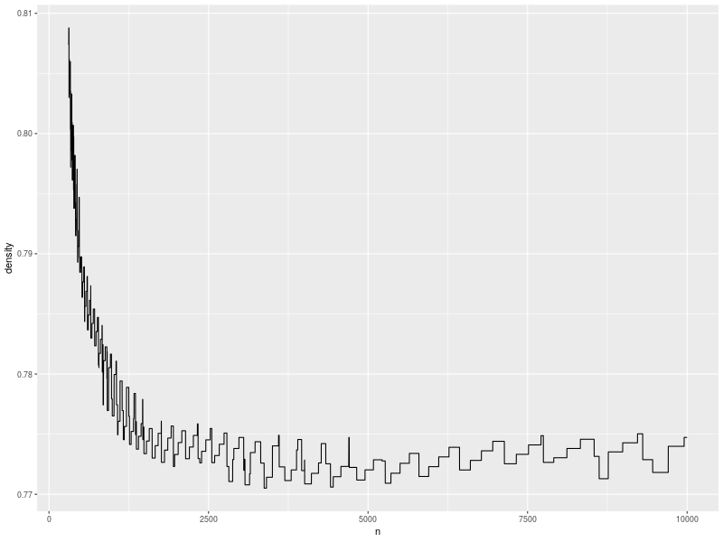
This curve roughly matches the shape of some my older purely numerical experiments with Robin Hood hashing. When the table is small (less than \(\approx 1000\)), \(\log n\) is a large fraction of \(n\), so the probability of finding a run of size \(s(n) = 5 \log\sb{2}\sp{3/2} n\) is low. When the table is much larger, the asymptotic result kicks in, and the probabiliy slowly shrinks. However, even around the worst case \(n \approx 4500\), we can exceed \(77\%\) density and only observe a run of length \(s(n)\) half the time.

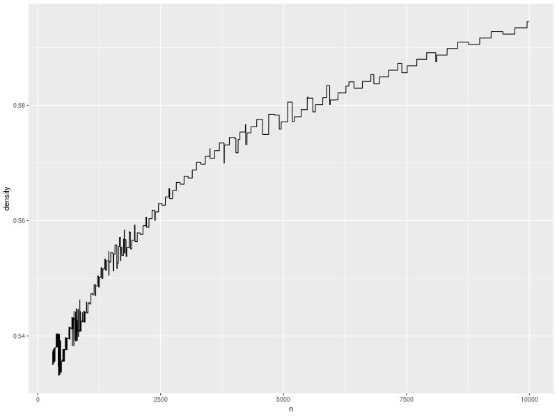
If we really don’t want to rehash, we can let \(\alpha = 10\sp{-10}\), which compresses the curve and shifts it down: the minimum value is now slightly above \(50\%\) density, and we can clearly see the growth in permissible density as the size of the table grows.

In practice, we can dynamically compute the worst-case displacement, which is always less than the longest run (i.e., less than \(s(n) = 5 \log\sb{2}\sp{3/2} n\)). However, having non-asymptotic bounds lets us write size-specialised code and know that its assumptions are likely to be satisfied in real life.

Bounding buffer sizes for operations on sorted hashed streams

I mentioned at the beginning of this post that we can also manipulate Robin Hood hash tables as sorted sets, where the sort keys are uniformly distributed hash values.

Let’s say we wished to merge the immutable source table S into the larger destination table D in-place, without copying all of D. For example, from

S = [2, 3, 4]
D = [1, 6, 7, 9, 10];

we want the merged result

D' = [1, 2, 3, 4, 6, 7, 9, 10].

The issue here is that, even with gaps, we might have to overwrite elements of D, and buffer them in some scratch space until we get to their final position. In this case, all three elements of S must be inserted between the first and second elements of D, so we could need to buffer D[1:4].

How large of a merge buffer should we reasonably plan for?

In general, we might have to buffer as many elements as there are in the smaller table of S and D. However, we’re working with hash values, so we can expect them to be distributed uniformly. That should give us some grip on the problem.

We can do even better and only assume that both sorted sets were sampled from the same underlying distribution. The key idea is that the rank of an element in S is equal to the value of S’s empirical distribution function for that element, multiplied by the size of S (similarly for D).

The amount of buffering we might need is simply a measure of the worst-case difference between the two empirical DFs: the more S get ahead of D, the more we need to buffer values of D before overwriting them (if we’re very unlucky, we might need a buffer the same size as S). That’s the two-sample Kolmogorov-Smirnov statistic, and we have simple bounds for that distance.

With probability \(1 - \alpha\), we’ll consume from S and D at the same rate \(\pm \sqrt{-\frac{(|S| + |D|) \ln \alpha}{2 |S| |D|}}\). We can let \(\alpha = 10\sp{-10}\) and pre-allocate a buffer of size

\[|S| \sqrt{-\frac{(|S| + |D|) \ln \alpha}{2 |S| |D|}} < \sqrt{\frac{23.03 |S| (|S| + |D|)}{2 |D|}}.\]

In the worst case, \(|S| = |D|\), and we can preallocate a buffer of size \(\sqrt{23.03 |D|} < 4.8 \sqrt{|D|}\) and only need to grow the buffer every ten billion (\(\alpha\sp{-1}\)) merge.

The same bound applies in a stream processing setting; I assume this is closer to what Frank had in mind when he brought up this question.

Let’s assume a “push” dataflow model, where we still work on sorted sets of uniformly distributed hash values (and the data tuples associated with them), but now in streams that generate values every tick. The buffer size problem now sounds as follows. We wish to implement a sorted merge operator for two input streams that generate one value every tick, and we can’t tell our sources to cease producing values; how much buffer space might we need in order to merge them correctly?

Again, we can go back to the Kolmogorov-Smirnov statistic. In this case however, we could buffer each stream independently, so we’re looking for critical values for the one-sided one-sample Kolmogorov-Smirnov test (how much one stream might get ahead of the hypothetical exactly uniform stream). We have recent (1990) simple and tight bounds for this case as well.

The critical values for the one-sided case are stronger than the two-sided two-sample critical values we used earlier: given an overflow probability of \(1 - \alpha\), we need to buffer at most \(\sqrt{-\frac{n \ln \alpha}{2}},\) elements. For \(\alpha = 10\sp{-20}\) that’s less than \(4.8 \sqrt{n}\).³ This square root scaling is pretty good news in practice: shrinking \(n\) to \(\sqrt{n}\) tends to correspond to going down a rung or two in the storage hierarchy. For example, \(10\sp{15}\) elements is clearly in the range of distributed storage; however, such a humongous stream calls for a buffer of fewer than \(1.5 \cdot 10\sp{8}\) elements, which, at a couple gigabytes, should fit in RAM on one large machine. Similarly, \(10\sp{10}\) elements might fill the RAM on one machine, but the corresponding buffer of less than half a million elements could fit in L3 cache, while one million elements could fill the L3, and 4800 elements fit in L1 or L2.

What I find neat about this (probabilistic) bound on the buffer size is its independence from the size of the other inputs to the merge operator. We can have a shared \(\Theta(\sqrt{n})\)-size buffer in front of each stream, and do all our operations without worrying about getting stuck (unless we’re extremely unlucky, in which case we can grow the buffer a bit and resume or restart the computation).

Probably of more theoretical interest is the fact that these bounds do not assume a uniform distribution, only that all the input streams are identically and independently sampled from the same underlying distribution. That’s the beauty of working in terms of the (inverse) distribution functions.

I don’t think there’s anything deeper

That’s it. Two cute tricks that use well-understood statistical distributions in hashed data structure and algorithm design. I doubt there’s anything to generalise from either bounding approach.

However, I definitely believe they’re useful in practice. I like knowing that I can expect the maximum displacement for a table of \(n\) elements with Robin Hood linear probing to be less than \(5 \log\sb{2}^{3/2} n\), because that lets me select an appropriate option for each table, as a function of that table’s maximum displacement, while knowing the range of displacements I might have to handle. Having a strong bound on how much I might have to buffer for stream join operators feels even more useful: I can pre-allocate a single buffer per stream and not think about efficiently growing the buffer, or signaling that a consumer is falling behind. The probability that I’ll need a larger buffer is so low that I just need to handle it, however inefficiently. In a replicated system, where each node picks an independent hash function, I would even consider crashing when the buffer is too small!

---