Back in November 2011, Takeru Ohta submitted a very nice patch to replace our (SBCL’s) in-place stable merge sort on linked lists with a simpler, much more efficient implementation. It took me until last May to whip myself into running a bunch of tests to estimate the performance improvements and make sure there weren’t any serious regression, and finally commit the patch. This post summarises what happened as I tried to find further improvements. The result is an implementation that’s linear-time on nearly sorted or reverse-sorted lists, around 4 times as fast on slightly shuffled lists, and up to 30% faster on completely shuffled lists, thanks to design choices guided by statistically significant effects on performance (… on one computer, my dual 2.8 GHz X5660).
I believe the approach I used to choose the implementation can be applied in other contexts, and the tiny tweak to adapt the sort to nearly-sorted inputs is simple (much simpler than explicitly detecting runs like Timsort), if a bit weak, and works with pretty much any merge sort.
A good starting point
The original code is reproduced below. The sort is parameterised on two functions: a comparator (test) and a key function that extracts the property on which data are compared. The key function is often the identity, but having it available is more convenient than having to pull the calls into the comparator. The sort is also stable, so we use it for both stable and regular sorting; I’d like to keep things that way to minimise maintenance and testing efforts. This implementation seems like a good foundation to me: it’s simple but pretty good (both in runtime and in number of comparisons). Trying to modify already-complicated code is no fun, and there’s little point trying to improve an implementation that doesn’t get the basics right.
1 2 3 4 5 6 7 8 9 10 11 12 13 14 15 16 17 18 19 | |
1 2 3 4 5 6 7 8 9 10 11 12 13 14 15 16 17 18 19 | |
There are a few obvious improvements to try out: larger base cases, recognition of sorted subsequences, converting branches to conditional moves, finding some way to avoid the initial call to length (which must traverse the whole linked list), … But first, what would interesting performance metrics be, and on what inputs?
Brainstorming an experiment up
I think it works better to first determine our objective, then the inputs to consider, and, last, the algorithmic variants to try and compare (decision variables). That’s more or less the reverse order of what’s usually suggested when defining mathematical models. The difference is that, in the current context, the space of inputs and algorithms are usually so large that we have to winnow them down by taking earlier choices into account.
Objective functions
A priori, three basic performance metrics seem interesting: runtimes, number of calls to the comparator, and number of calls to the key functions. On further thought, the last one doesn’t seem useful: if it really matters, a schwartzian transform suffices to reduce these calls to a minimum, regardless of the sort implementation.
There are some complications when looking at runtimes. The universe
of test and key functions is huge, and the sorts can be inlined, which
sometimes enables further specialisation on the test and key. I’ve
already decided that calls to key don’t matter directly. Let’s
suppose it’s very simple, the identity function. The number of
comparisons will correlate nicely with performance when comparisons
are slow. Again, let’s suppose that the comparator is simple, a
straight < of fixnums. The performance of sorts, especially with a
trivial key and a simple comparator, can vary a lot depending on
whether the sort is specialised or not, and both cases are relevant in
practice. I’ll have to test for both cases: inlined comparator and
key functions, and generic sorts with unknown functions.
This process lead to a set of three objective functions: the number of calls to the comparator, the runtime (number of cycles) of normal, generic sort, and the number of cycles for a specialised sort.
Inputs
The obvious thing to vary in the input (the list to sort) is the length of the list. The lengths should probably span a wide range of values, from short lists (e.g. 32 elements) to long ones (a few million elements). Programs that are sort-bound on very long lists should probably use vectors, if only around the sort, and then invest in a sophisticated sort.
In real programs, sort is sometimes called on nearly sorted or reverse-sorted sequences, and it’s useful to sort such inputs faster, or with fewer comparisons. However, it’s probably not that interesting if the adaptivity comes at the cost of worse performance on fully shuffled lists. I decided to test on sorted and fully shuffled inputs. I also interpolated between the two by flipping randomly-selected subranges of the list a few times.
Finally, linked lists are different than vectors in one key manner: contiguous elements can be arbitrarily scattered around memory. SBCL’s allocation scheme ensures that consecutively-allocated objects will tend to be located next to each other in memory, and the copying garbage collector is hacked to copy the spine of cons lists in order. However, a list can still temporarily exhibit bad locality, for example after an in-place sort. Again, I decided to go for ordered conses, fully scattered conses (only the conses were shuffled, not the list’s values), and to interpolate, this time by swapping randomly-selected pairs of consecutive subranges a couple times.
Code tweaks
The textbook way to improve a recursive algorithm is to increase the base cases’ sizes. In the initial code the base case is a sublist of size one; such a list is trivially sorted. We can easily increase that to two (a single conditional swap suffices), and an optimal sorting network for three values is only slightly more complicated. I decided to stop there, with base cases of size one to three. These simple sorts are implemented as a series of conditional swaps (i.e. pairs of max/min computations), and these can be executed branch-free, with only conditional moves. There’s a bit of overhead, and conditional moves introduce more latency than well predicted branches, but it might be useful for the specialised sort on shuffled inputs, and otherwise not hurt too much.
The merge loop could cache the result of calls to the key functions. This won’t be useful in specialised sorts, and won’t affect the number of comparisons, but it’ll probably help the generic sort without really affecting performance otherwise.
With one more level of indirection, the merge loop can be branch-free:
merge-one can be executed on references to the list heads, and these
references can be swapped with conditional moves. Again, the
additional complexity makes it hard to guess if the change would be a
net improvement.
Like I hinted back in May, we can accelerate the sort on pre-sorted inputs by keeping track of the last cons in each list, and tweaking the merge function: if the first value in one list is greater than (or equal to) the last in the other, we can directly splice them in order. Stability means we have to add a bit of complexity to handle equal values correctly, but nothing major. With this tiny tweak, merge sort is linear-time on sorted or reverse-sorted lists (the recursive step is constant-time, and merge sort recurses on both halves); it also works on recursively-processed sublists, and the performance is thus improved on nearly-sorted inputs in general. There’s little point going through additional comparisons to accelerate the merger of two tiny lists; a minimal length check is in order. In addition to the current version, without any quick merge, I decided to try quick merges when the length of the two sublists summed to at least 8, 16 or
- I didn’t try limits lower than 8 because any improvement would probably be marginal: trying to detect opportunities for quicker merge introduces two additional comparisons when it fails.
Finally, I tried to see if the initial call to length (which has to
traverse the whole list) could be avoided, e.g. by switching to a
bottom-up sort. The benchmarks I ran in May made me realise that’s
probably a bad idea. Such a merge sort almost assuredly has to split
its inputs in chunks of power of two (or some other base) sizes.
These splits are suboptimal on non-power-of-two inputs; for example,
when sorting a list of length (1+ (ash 1 n)), the final merge is
between a list of length (ash 1 n) and a list of length … one.
Knowing the exact length of the list means we can split optimally on
recursive calls, and that eliminates bumps in runtimes and in the
number of comparisons around “round” lengths.
How can we compare all these possibilities?
I usually don’t try to do anything clever, and simply run a large number of repetitions for all the possible implementations and families of inputs, and then choose a few interesting statistical tests or sic an ANOVA on it. The problem is, I’d maybe want to test with ten lengths (to span the wide range between 32 and a couple million), a couple shuffledness values (say, four, between sorted and shuffled), a couple scatteredness values (say, four, again), and around 48 implementations (size-1 base case, size-3 base case, size-3 base case with conditional moves, times cached or uncached key, times branchful or branch-free merge loop, times four possibilities for the quick merge). That’s a total of 7680 sets of parameter values. If I repeated each possibility 100 times, a reasonable sample size, I’d have to wait around 200 hours, given an average time of 1 second/execution (a generous estimate, given how slow shuffling and scattering lists can be)… and I’d have to do that separately when testing for comparison counts, generic sort runtimes and specialised sort runtimes!
I like working on SBCL, but not enough to give its merge sort multiple CPU-weeks.
Executing multiple repetitions of the full cross product is overkill: that actually gives us enough information to extract information about the interaction between arbitrary pairs (or arbitrary subsets, in fact) of parameters (e.g. shuffledness and the minimum length at which we try to merge in constant-time). The thing is, I’d never even try to interpret all these crossed effects: there are way too many pairs, triplets, etc. I could instead try to determine interesting crosses ahead of time, and find a design that fits my simple needs.
Increasing the length of the list will lead to longer runtimes and more comparisons. Scattering the cons cells around will also slow the sorts down, particularly on long lists. Hopefully, the sorts are similar enough to be affected comparably by the length of the list and by how its conses are scattered in memory.
Pre-sorted lists should be quicker to sort than shuffled ones, even without any clever merge step: all the branches that depend on comparisons are trivially predicted. Hopefully, the effect is more marked when sorted pairs of sublists are merged in constant time.
Finally, the interaction between the remaining algorithmic tweaks is pretty hard to guess, and there are only 12 combinations. I feel it’s reasonable to cross the three parameter sets.
That’s three sets of crossed effects (length and scatteredness, shuffledness and quick merge switch-over, remaining algorithmic tweaks), but I’m not interested in any further interaction, and am actually hoping these interactions are negligible. A Latin square design can help bring the sample to a much more reasonable size.
Quadrata Latina pro victoria
An NxN Latin square is a square of NxN cells, with one of N symbols in each cell, with the constraint that each symbol appears once in each row and column; it’s a relaxed Sudoku.
When a first set of parameters values is associated with the rows, a second with the columns, and a third with the symbols, a Latin square defines N^2 triplets that cover each pair of parameters between the three sets exactly once. As long as interactions are absent or negligible, that’s enough information to separate the effect of each set of parameters. The approach is interesting because there are only N^2 cells (i.e. trials), instead of N^3. Better, the design can cope with very low repetition counts, as low as a single trial per cell.
Latin squares are also fairly easy to generate. It suffices to fill the first column with the symbols in arbitrary order, the second in the same order, rotated by one position, the third with a rotation by two, etc. The square can be further randomised by shuffling the rows and columns (with Fisher-Yates, for example). That procedure doesn’t sample from the full universe of Latin squares, but it’s supposed to be good enough to uncover pairwise interactions.
Latin squares only make sense when all three sets of parameters are the same size. Latin rectangles can be used when one of the sets is smaller than the two others, by simply removing rows or columns from a random Latin square. Some pairs are then left unexplored, but the data still suffices for uncrossed linear fits, and generating independent rectangles helps cover more possibilities.
I’ll treat all the variables as categorical, even though some take numerical values: it’ll work better on non-linear effects (and I have no clue what functional form to use).
Optimising for comparison counts
Comparison counts are easier to analyse. They’re oblivious to micro-optimisation issues like conditional moves or scattered conses, and results are deterministic for fixed inputs. There are much fewer possibilities to consider, and less noise.
Four values for the minimum length before checking for constant-time merger (8, 16, 32 or never), and ten shuffledness values (sorted, one, two, five, ten, 50, 100, 500 or 1000 flips, and full shuffle) seem reasonable; when the number of flips is equal to or exceeds the list length, a full shuffle is performed instead. That’s 40 values for one parameter set.
There are only two interesting values for the remaining algorithmic tweaks: size-3 base cases or not (only size-1).
This means there should be 40 list lengths to balance the design. I chose to interpolate from 32 to 16M (inclusively) with a geometric sequence, rounded to the nearest integer.
The resulting Latin rectangles comprise 80 cells. Each scenario was repeated five times (starting from the same five PRNG states), and 30 independent rectangles were generated. In total, that’s 12 000 executions. The are probably smarter ways to do this that better exploit the fact that there are only two algorithmic tweaks variants; I stuck to a very thin Latin rectangle to stay closer to the next two settings. Still, a full cross product with 100 repetitions would have called for 320 000 executions, nearly 30 times as many.
I wish to understand the effect of these various parameters on the number of times the comparison function is called to sort a list. Simple models tend to suppose additive effects. That doesn’t look like it’d work well here. I expect multiplicative effects: enabling quick merge shouldn’t add or subtract to the number of comparisons, but scale it (hopefully by less than one). A logarithmic transformation will convert these multiplications into additions. The ANOVA method and the linear regression I’ll use are parametric methods that suppose that the mean of experimental noise roughly follows a normal distribution. It seems like a reasonable hypothesis: variations will be caused by a sum of many small differences caused by the shuffling, and we’re working with many repetitions, hopefully enough for the central limit theorem to kick in.
The Latin square method also depends on the absence of crossed interactions between rows and columns, rows and symbols, or columns and symbols. If that constraint is violated, the design is highly vulnerable to Type I errors: variations caused by interactions between rows and columns could be assigned to rows or columns, for example.
My first step is to look for such interaction effects.
1 2 3 4 5 6 7 8 9 10 11 12 13 14 15 16 17 18 | |
The main effects are statistically significant (in order, list length,
shuffling and quick merge limit, and the algorithmic tweaks), with p <
2e-16. That’s reassuring: the odds of observing such results if they
had no effects are negligible. Two of the pairs are, as well. Their
effects, on the other hand, don’t seem meaningful. The Sum Sq
column reports how much of the variance in the data set is explained
when the parameters corresponding to each row (one for each degree of
freedom Df) are introduced in the fit. Only the
Size.Scatter:Shuffle.Quick row really improves the fit, and that’s
with 1159 degrees of freedom; the mean improvement in fit, Mean Sq
(per degree of freedom) is tiny.
The additional assumption that interaction effects are negligible seems reasonably satisfied. The linear model should be valid, but, more importantly, we can analyse each set of parameters independently. Let’s look at a regression with only the main effects.
1 2 3 4 5 6 7 8 9 10 11 12 13 | |
The fit is only slightly worse than with pairwise interactions. The coefficient table follows. What we see is that half of the observations fall within 12% of the linear model’s prediction (the worst case is off by more than 100%), and that nearly all the coefficients are statistically significantly different than zero.
1 2 3 4 5 6 7 8 9 10 11 12 13 14 15 16 17 18 19 20 21 22 23 24 25 26 27 28 | |
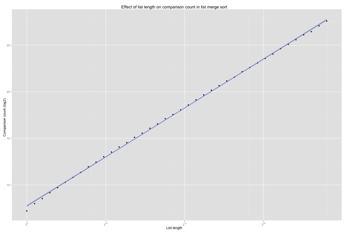
The Size.Scatter coefficients are plotted below. The number of comparison grows with the length of the lists. The logarithmic factor shows in the curve’s slight convexity (compare to the linear interpolation in blue).
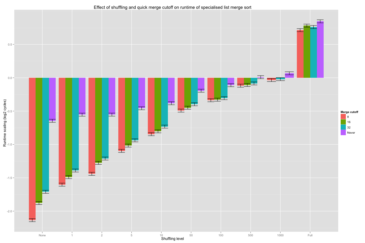
The Shuffle.Quick values are the coefficients for the crossed effect of the level of shuffling and the minimum length (cutoff) at which constant-time merge may be executed; their values are reported in the next histogram, with error bars corresponding to one standard deviation. Hopefully, a shorter cutoff lowers the number of comparisons when lists are nearly pre-sorted, and doesn’t increase it too much when lists are fully shuffled. On very nearly sorted lists, looking for pre-sorted inputs as soon as eight or more values are merged divides the number of comparisons by a factor of 4 (these are base-2 logarithms), and the advantage smoothly tails off as lists are shuffled better. Overall, cutting off at eight seems to never do substantially worse than the other choices, and is even roughly equivalent to vanilla merges on fully shuffled inputs.
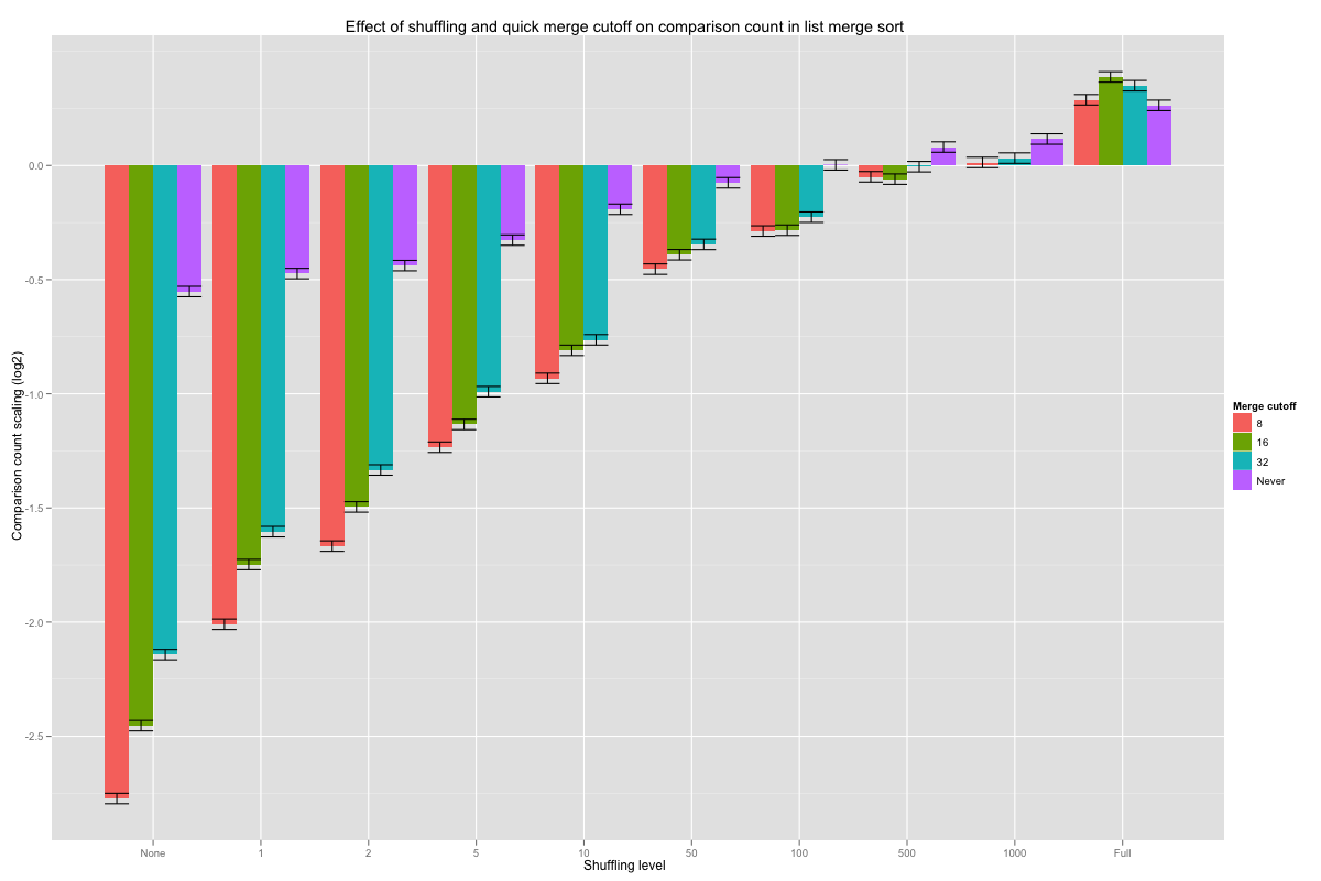
The coefficient table tells us that nearly all of the Shuffle.Quick coefficients are statistically significant. The statistical significance values are for a null hypothesis that each of these coefficients is actually zero: the observation would be extremely unlikely if that were the case. That test tells us nothing about the relationship between two coefficients.
Comparing differences with standard deviations helps us detect hugely significant difference, but we can use statistical tests to try and make finer distinctions. Tukey’s Honest Significant Difference (HSD) method gives intervals on the difference between two coefficients for a given confidence level. For example, the 99.99% confidence interval between cutoff at 8 and 32 on lists that were flipped 50 times is [-0.245, -0.00553]. This result means that, if the hypotheses for Tukey’s HSD method are satisfied, the probability of observing the results I found is less than .01% when the actual difference in effect between cutoff at 8 and 32 is outside that interval. Since even the upper bound is negative, it also means that the odds of observing the current results are less than .01% if the real value for cutoff at 8 isn’t lower than that of cutoff at 32: it’s pretty sure that looking for quick merges as early as length eight pays off compared to only doing so for merges of length 32 or more. One could also just prove that’s the case. Overall, cutting off at length eight results in fewer comparisons than the other options at nearly all shuffling levels (with very high confidence), and the few cases cases it doesn’t aren’t statistically significant at a 99.99% confidence level – of course, absence of evidence isn’t evidence of absence, but the differences between these estimates tend to be tiny anyway.
The last row, Leaf.Cache.BranchMergeTxFxT, reports the effect of adding base cases that sort lists of length 2 and 3. Doing so causes 4% more comparisons. That’s a bit surprising: adding specialised base cases usually improves performance. The issue is that the sorting networks are only optimal for data-oblivious executions. Sorting three values requires, in theory, 2.58 (\(\lg 3!\)) bits of information (comparisons). A sorting network can’t do better than the ceiling of that, three comparisons, but if control flow can depend on the comparisons, some lists can be sorted in two comparisons.
It seems that, if we wish to minimise the number of comparisons, I should avoid sorting networks for the size-3 base case, and try to detect opportunities for constant-time list merges. Doing so as soon as the merged list will be of length eight or more seems best.
Optimising the runtime of generic sorts
I decided to keep the same general shape of 40x40xM parameter values when looking at the cycle count for generic sorts. This time, scattering conses around in memory will affect the results. I went with conses laid out linearly, 10 swaps, 50 swaps, and full randomisation of addresses. These 4 scattering values leave 10 list lengths, in a geometric progression from 32 to 16M. Now, it makes sense to try all the other micro-optimisations: trivial base case or base cases of size up to 3, with branches or conditional moves (3 choices), cached calls to key during merge (2 choices), and branches or conditional moves in the merge loop (2 choices). This calls for Latin rectangles of size 40x12; I generated 10 rectangles, and repeated each cell 5 times (starting from the same 5 PRNG seeds). In total, that’s 24 000 executions. A full cross product, without any repetition, would require 19 200 executions; the Latin square design easily saved a factor of 10 in terms of sample size (and computation time) for equivalent power.
I’m interested in execution times, so I generated the inputs ahead of time, before sorting them; during both generation and sorting, the garbage collector was disabled to avoid major slowdowns caused by the mprotect-based write barrier.
Again, I have to apply a logarithmic transformation for the additive model to make sense, and first look at the interaction effects. There’s a similar situation as the previous section on comparison counts: one of the crossed effects is statistically significant, but it’s not overly meaningful. A quick look at the coefficients reveals that the speed-ups caused by processing nearly-sorted lists in close to linear time are overestimated on short lists and slightly underestimated on long ones.
1 2 3 4 5 6 7 8 9 10 11 12 13 14 15 16 17 18 | |
We can basically read the ANOVA with only main effects by skipping the rows corresponding to crossed effects and instead adding their values to the residuals. There are statistically significant coefficients in there, and they’re reported below. Again, I’m quite happy to be able to examine each set of parameters independently, rather than having to understand how, e.g., scattering cons cells around affects quick merges differently than the vanilla merge. Maybe I just didn’t choose the right parameters, or was really unlucky; I’m just trying to do the best I can with induction.
1 2 3 4 5 6 7 8 9 10 11 12 13 14 15 16 17 18 19 20 21 22 23 24 25 26 27 28 29 30 31 32 33 34 35 36 37 38 39 40 41 42 43 44 45 46 47 | |
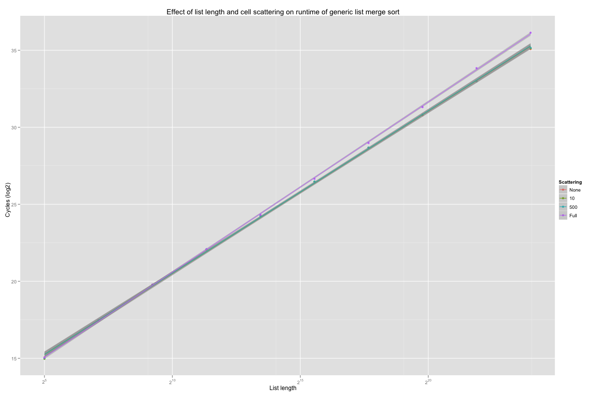
The coefficients for list length crossed with scattering level are plotted below. Sorting seems to be slower on longer list (surprise!), especially when the cons cells are scattered; sorting long scattered lists is about twice as slow as sorting nicely laid-out lists of the same length. The difference between linear and slightly scattered lists isn’t statistically significant.
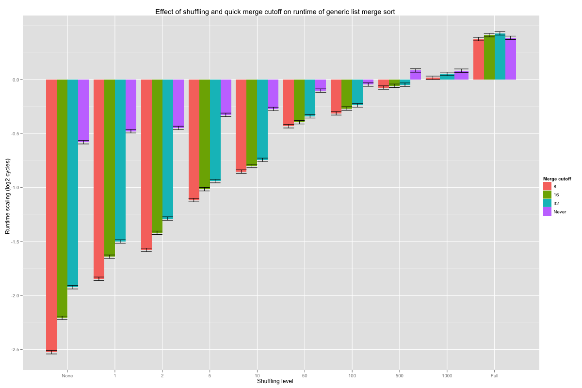
Just as with comparison counts, sorting pre-sorted lists is faster, with or without special logic. Looking for sorted inputs before merging pays off even on short lists, when the input is nearly sorted: the effect of looking for pre-sorted inputs even on sublists of length eight is consistently more negative (i.e. reduces runtimes) than for the other cutoffs. The difference is statistically significant at nearly all shuffling levels, and never significantly positive.
Finally, the three algorithmic tweaks. Interestingly, the coefficients tell us that, overall, the additional overhead of the branch-free merge loop slows it down by 5%. The fastest combination seems to be larger base cases, with or without conditional moves (C or T), cached calls to key (T), and branchful merge loop (T); the differences are statistically significant against nearly all other combinations, except FxTxT (no leaf sort, cached key, and branchful merge loop). Compared with the current code (FxFxT), the speed up is on the order of 5%, and at least 2% with 99.99% confidence.
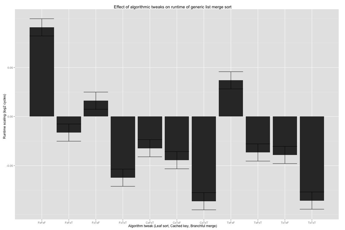
If I want to improve the performance of generic sorts, it looks like I want to test for pre-sorted inputs when merging into a list of length 8 or more, probably implement larger base cases, cache calls to the key function, and keep the merge loop branchful.
Optimising the runtime of specialised sorts
I kept the exact same plan as for generic sorts. The only difference is that independent Latin rectangles were re-generated from scratch. With the overhead from generic indirect calls removed, I’m hoping to see more important effects from the micro-optimisations.
1 2 3 4 5 6 7 8 9 10 11 12 13 14 15 16 17 18 19 | |
Here as well, all the main and crossed effects are statistically significant. The effect of the micro-optimisations (Leaf.Cache.BranchMerge) are now about as influential as the fast merge minimum length. It’s also even more clear that the crossed effects are much less important than the main ones, and that it’s probably not too bad to ignore the former.
1 2 3 4 5 6 7 8 9 10 11 12 13 14 15 16 17 18 19 20 21 22 23 24 25 26 27 28 29 30 31 32 33 34 35 36 37 38 39 40 41 42 43 44 45 46 47 48 | |
The general aspect of the coefficients is pretty much the same as for generic sorts, except that differences are amplified now that the constant overhead of indirect calls is eliminated.
The coefficients for crossed list length and scattering level coefficients are plotted below. The graph shows that fully shuffling long lists around slows sort down by a factor of 8. The initial check for crossed effect gave good reasons to believe that this effect is fairly homogeneous throughout all implementations.

Checking for sorted inputs before merge still helps, even on short lists (of length 8 or more). In fact even on completely shuffled lists, looking for quick merge on short lists very probably accelerates the sort compared to not looking for pre-sorted inputs, although the speed up compared to other cutoff values isn’t significant to a 99.99% confidence level.
The key function is the identity, and is inlined into nothing in these measurements. It’s not surprising that the difference between cached and uncached key values is tiny. The versions with larger base cases (C or T) sorts, and branchful merge are quicker than the others at 99.99% confidence level; compared to the initial code, they’re at least 13% faster with 99.99% confidence.
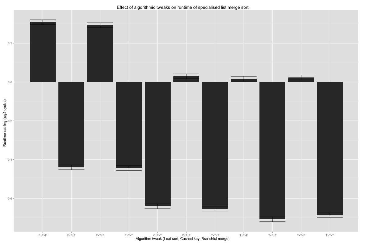
When the sort is specialised, I probably want to use a merge function that checks for pre-sorted inputs very early, to implement larger base cases (with conditional moves or branches), and to keep the merge loop branchful.
Putting it all together
Comparison counts are minimised by avoiding sorting networks, and by enabling opportunistic constant-time merges as early as possible. Generic sorts are fastest with larger base cases (with or without branches), cached calls to the key function, a branchful merge loop and early checks for constant-time merges. Specialised sorts are, similarly, fastest with larger base cases, a branchful merge loop and early checks when merging (without positive or negative effect from caching calls to the key function, even if it’s the identity).
Overall, these result point me toward one implementation: branchful size-2 and size-3 base cases that let me avoid redundant comparisons, cached calls to the key function, branchful merge loop, and checks for constant-time merges when the result is of length eight or more.
The compound effect of these choices is linear time complexity on sorted inputs, speed-ups (and reduction in comparison counts) by factors of 2 to 4 on nearly-sorted inputs, and by 5% to 30% on shuffled lists.
The resulting code follows.
1 2 3 4 5 6 7 8 9 10 11 12 13 14 15 16 17 18 19 20 21 22 | |
1 2 3 4 5 6 7 8 9 10 11 12 13 14 15 16 17 18 19 20 21 22 23 24 25 26 27 28 29 30 31 32 33 | |
1 2 3 4 5 6 7 8 9 10 11 12 13 14 15 16 17 18 19 20 21 22 23 24 25 26 27 28 29 30 31 32 33 34 35 36 37 38 39 40 41 42 43 | |
It’s somewhat longer than the original, but not much more complicated: the extra code mostly comes from the tedious but simple leaf sorts. Particularly satisfying is the absence of conditional move hack: SBCL only recognizes trivial forms, and only on X86 or X86-64, so the code tends to be ugly and sometimes sacrifices performance on other platforms. SBCL’s bad support for conditional moves may explain the lack of any speed up from converting branches to select expressions: the conditional swaps had to be implemented as pairs of independent test with T/NIL and conditional moves. Worse, when the comparison is inlined, an additional conditional move converted the result of the integer comparison to a boolean value; in total, three pairs of comparison/conditional move were then executed instead of one comparison and two conditional moves. Previous work [PDF] on out-of-place array merge sort in C found it useful to switch to conditional move-based merge loop and sorting networks. Some of the difference is probably caused by SBCL’s weaker code generation, but the additional overhead inherent to linked list manipulations (compared to linear accesses in arrays) may also play a part.
Another code generation issue is caused by the way the initial version called the comparison function in exactly one place. This meant that arbitrary comparators would almost always be inlined in the specialised sort’s single call site. We lose that property with accelerated merge and larger base cases. That issue doesn’t worry me too much: functions can be declared inline explicitly, and the key function was already called from multiple sites.
I’m a bit surprised that neither the sorting networks nor the merge loop were appreciably sped-up by rewriting them with conditional moves. I’m a lot more surprised by the fact that it pays off to try and detect pre-sorted lists even on tiny merges, and even when the comparator is inlined. The statistical tests were useful here, with results that defy my initial expectations and let me keep the code simpler. I would be pleasantly surprised if complex performance improvement patches, in SBCL and otherwise, went through similar testing. Code is a long-term liability, and we ought to be convinced the additional complexity is worth the trouble.
Independently of that, the Latin square design was very helpful: it easily saved me a couple CPU-weeks, and I can see myself using it regularly in the future. The approach only works if we already have a rough (and simple) performance model, but I have a hard time interpreting complex models with hundreds of interacting parameters anyway. Between a simplistic, but still useful, model and a complex one with a much stronger fit, I’ll usually choose the former… as long as I can be fairly certain the simple model isn’t showing me a mirage.
More generally, research domains that deal with the real world have probably already hit the kind of scaling issues we’re now facing when we try to characterise how computers and digital systems function. Brute forcing is easier with computers than with interns, but it can still pay off to look elsewhere.