Programmers tend to like round numbers, i.e. powers of two. So do hardware designers. Sadly, this shared value doesn’t always work to our advantage. One common issue is that of cache line aliasing induced by alignment.

Binary search suffers from a related ailment when executed on medium or large vectors of almost power-of-two size (in bytes), but it can be cured. Once that is done, searching a sorted vector can be as fast as searches with a well-tuned hash table, for a few realistic access patterns.

The task is interesting to me because I regularly work with static, or almost static, sets: sets for which there’s a majority of lookups, while updates are either rare or batchable. For such sets, the improved performance of explicit balanced search trees on insertions is rarely worth the slowdown on lookups, nor the additional space usage. Replacing binary search with slightly off-center binary or quaternary (four-way) searches only adds a bit more code to provide even quicker, more consistent lookup times.

Analyze this

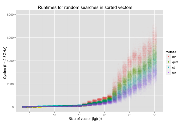
The following jittered scatterplot reports the runtimes, on my dual 2.8 GHz X5660, for binary searches to the first value in a single sorted vector of size 16 to 1G elements (32-bit unsigneds), and is overlaid with the median in green. For each power-of-two size, the benchmark program was executed 10 times, with 100 000 binary searches per execution (and each search was timed individually, with rdtscp). Finally, NUMA effects were eliminated by forcing the processes to run and acquire memory from the same un-loaded node. 1 000 000 points are hard to handle, so the plot is only based on a .1% random sample (i.e. 1 000 points for each size).

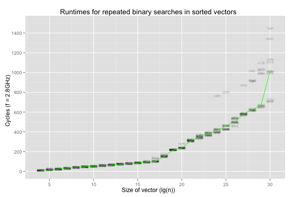
Two things bother me here. The performance degrades much more quickly when \(\lg(n)\geq 17\) (i.e. the size exceeds 512 KB), but, worse, it shows a lot of variation on larger vectors. The variation seems more critical to me. Examining the data set reveals that the variation is purely inter-execution: each set of 100 000 repetitions shows nearly constant timings.

The degradation after \(\lg(n)=17\) is worrying because drops in performance when the input is 512 KB or larger looks a lot like a cache issue. However, the workload is perfectly cachable: even on vectors of 1G values, binary search is always passed the same key and vector, and thus always reads from the same 30 locations. This should have no trouble fitting in L1 cache, for the whole range of sizes considered here.

The variation is even stranger. It happens between executions of identical binaries for a deterministic program, on the same machine and OS, but never in a single execution. The variation makes no sense. If the definition of insanity is doing the same thing over and over again and expecting different results, contemporary computers are quite ill. Worse, the variation would never have been uncovered by repetitions in a single process. I was lucky to look at the results from multiple executions, otherwise I could easily have concluded that binary search for the same element in a vector of 1G 32-bit elements almost always takes around 700 cycles, or almost always 1400ish cycles.

What’s behind the speed bump and the extreme variations?

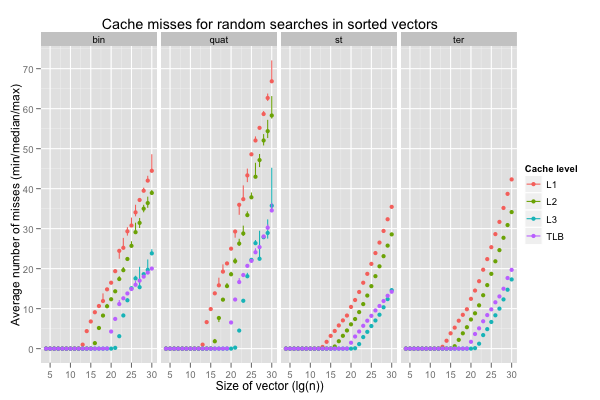
The next graph reports the number of cache misses at the first, second, third and translation lookaside buffer levels. The average count per search over 100 000 repetitions were recorded in 10 independent executions for each size. The points correspond to medians of ten average counts, and the vertical lines span the minimum and maximum counts.

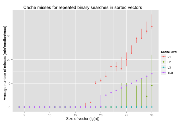
The miss counts between executions are pretty much constant for L3 and TLB, and reasonably consistent for L1. L1 and TLB misses seem to cause the slowdown, even though the working sets are tiny. L2 misses on \(\lg(n)\geq 24\) are all over the place, and seem to be behind the variability.

Yet another meaning for aliasing

Something’s wrong with the caches. We’ve found an issue with classic binary search – that splits the range at each iteration in the middle – on vectors of (nearly-)power-of-two size, in bytes.

Nearly all (cacheful) processors to this day map memory addresses to cache locations by taking the modulo with a power of two. For example, with 1K cache lines of 64 bytes, 0xabcd = 43981 is mapped to \((43981\div 64)\mod 1024\). This is as simple to understand as it is to implement: just select a short range of bits from the address. It also has the side effect that nicely-aligned data will often map to the same cache lines. Two vectors of 64KB each, allocated at 0x10000 and 0x20000, have the unfortunate property that, for each index, the data at that index in both vectors will map to the same cache lines in a direct-mapped cache with 1024 lines of 64 bytes each. When only one cache line is allowed per location, iterating through both vectors in the same loop will ping-pong the data from both vectors between cache and memory, without ever benefiting from caching. The addresses alias each other, and that’s bad.

There are workarounds, on both the hardware and software sides.

Current X86s tend to avoid fast, direct-mapped, caches even at the first level: set-associative caches are designed to handle a small number of collisions (like fixed-size buckets in hash tables), from 2-4 in the fastest levels to 8, 16 or more for last level caches. This ensures that a program can access two similarly-aligned vectors in lockstep, without having each access to one vector evicting cached data from the other. It’s far from perfect: a 2-way associative cache enables a loop over two vectors to work fine, but, as soon as the loop iterates over three or more vectors, it suddenly becomes much slower. Arguably more robust solutions involving prime moduli, hash functions, or other clever address-to-cache-line mappings have been proposed since the 80’s (this [pdf] is a recent one, with a nice set of references to older work), but I don’t think any has ever gained traction.

On the software end, smart memory allocators try to alleviate the problem by offsetting large allocations away from the beginning of pages. Inserting a variable number of cache lines as padding (before allocated data) minimises the odds that vector traversals suffer from aliasing. Sadly, that’s not yet the case for SBCL. In fact, as well as pretty much guaranteeing that large vectors will alias each other, SBCL’s allocator also makes cache-aware traversals hard to write: the allocator aligns the vector’s header (two words for a length and type descriptor) rather than its data. That’s the kind of consideration that is too easily disregarded when designing a runtime system; getting it right after the fact probably isn’t hard, but may call for some unsavory hacks.

Aliasing in binary search

Binary search doesn’t involve lockstep traversals over multiple vectors. However, when the vector to search into is of power-of-two length (or almost), the first few accesses are to similarly-aligned addresses (e.g. in a 64KB vector of 32-bit values, it could access indices 0x8000, 0x4000, 0x2000, 0x1000, etc.). Similar issues crop up when working with power-of-two-sized matrices, or when bit-reversing a vector. We can easily convince ourselves that the access patterns will be similarly structured when binary searching vectors of size slightly (on the order of one or two cache lines) shorter or longer than powers of two.

On my X5660, the L1D cache has 512 lines of 64 bytes each, L2 4096 lines, and L3 196608 lines (12 MB). Crucially, the L1 and L2 caches are 8-way set-associative, and the L3 16-way. The TLBs are 4-way associative, and the first level has 64 entries and the second 512.

The number of L1 cache misses explodes on vectors of 512K elements and more. The L1D is designed so that only contiguous ranges of \(64\times 512\div 8 = 4 \textrm{KB}\) (one normal page) can be cached without collisions. For \(\lg(n)=19\), binary search needs 10 reads that all map to the same set of cache lines before reducing the candidate range below 4 KB. Once the first level cache’s 8-way associativity has been exhausted, binary search on a vector of 512K 4-byte elements still has to read two more locations before hitting a different set (bucket) of cache lines. This accounts for the L1 misses: so many reads are to locations that map to the same cache lines that a tiny working set exceeds the L1D’s wayness. To make things worse, LRU-style replacement strategy are useless. We have a similar issue on TLB misses (plus, filling the TLB on misses means additional data cache misses to walk the page table).

In contrast, the L3 is large enough and has a high-enough associativity to accomodate the binary search.

That leaves the wildly-varying miss counts for the second level cache. The L1D cache is able to fullfill some reads, which explains why L2 misses only appear on larger searches. The variation is surprising. What happens is that, on the X5660, caching depends on physical memory addresses, and those are fully under the OS’s control and hidden from userspace. The exception is the L1D cache, in which the sets only cover 4 KB (one normal page). It’s just small enough that the bits used to determine the set are always the same for both virtual and physical addresses, and the CPU can thus perform part of the lookup in parallel with address translation. This hidden variable explains the large discrepancies in L2 miss counts that is then reflected in runtimes. Sometimes the OS hands us a range of physical pages that works well for our workloads, other times it doesn’t. Not only is there nothing we can do about it, but we also can’t even know about it, except indirectly, or with unportable hacks. Finally, the OS can’t change the mapping without copying data, so that happens very rarely, and memory allocators tend to minimise syscalls by keeping previously-allocated address space around. In effect, an application that’s unlucky in its allotment of physical addresses can do little about it and can’t really tell except by logging bad performance.

Searching for a solution

Classic binary search on power-of-two sized vectors is a pathological case for small (i.e. fast) caches and TLBs, and its performance varies a lot based on physical address allocation, something over which we have no control. The previous section only covered a trivial case, and real workloads will be even worse. We could try to improve performance and consistency by introducing padding, either after each element or between chunks of elements, but I’d prefer a different solution that preserves the optimal density and simplicity of sorted vectors.

There are many occurrences of two as a magic number in our test cases. On the hardware side, cache lines are power-of-two sizes, as are L1 and L2 set (buckets) counts. On the software side, each unsigned is 4-bytes long, the vectors are of power-of-two lengths, and binary search divides the size of the candidate range by two. There’s little we can do about hardware, and changing our interface to avoid round element sizes or counts isn’t always possible. The only remaining knob to improve the performance and consistency of binary search is the division factor.

The successor of two is three. How can we divide a power-of-two size vector in three subranges? One way is to vary the size of the subdivided range, and keep track of it at runtime. There’s a simpler workaround: it’s all right, if suboptimal, to search over a wider range than strictly necessary, as long as no out-of-bounds access is performed. For example, a vector of length 8 can be split at indices \(\lceil 8/3\rceil = 3\) and \(8-3 = 5\); the next range will be either [0, 3), [3, 5) or [5, 8). The middle range is of length 2 rather than 3, but the search is still correct if it’s executed over [3, 6) instead of [3, 5).

Ternary search functions were generated for each vector size; when the last range was of length 2, a binary search step was executed instead. The example below is for a vector of length 32K. It implements a lower bound search, assuming that the key is greater than or equal to the first element in the vector (otherwise, the first element is spuriously considered as the lower bound).

1
2
3
4
5
6
7
8
9
10
11
12
13
14
15

size_t t_15 (unsigned key, unsigned * vector)
{
     unsigned * base = vector;
     TERNARY(10923u, 21845u);       /*      32768 -> 10923      */
     TERNARY(3641u, 7282u);         /*      10923 -> 3641       */
     TERNARY(1214u, 2427u);         /*       3641 -> 1214       */
     TERNARY(405u, 809u);           /*       1214 -> 405        */
     TERNARY(135u, 270u);           /*        405 -> 135        */
     TERNARY(45u, 90u);             /*        135 -> 45         */
     TERNARY(15u, 30u);             /*         45 -> 15         */
     TERNARY(5u, 10u);              /*         15 -> 5          */
     TERNARY(2u, 3u);               /*          5 -> 2          */
     BINARY(1u);                    /*          2 -> 1          */
     return base-vector;
}

Similar code was generated for binary searches. We still have to define the expansion for each TERNARY or BINARY step.

BINARY is easy: we simply reuse the logic from the previous post on binary search and branch mispredictions.

1
2
3
4
5
6

#define BARRIER do { __asm__ volatile("" ::: "memory"); } while (0)

#define BINARY(I) do {                                          \
                base = ((base)[I] <= key)?base+I:base;          \
                BARRIER;                                        \
        } while (0)

The compiler barrier was the most straightforward way I found to prevent gcc from noticing potentially-redundant accesses and trying to optimise them away by inserting branches.

TERNARY present a choice: do we try to expose memory-level parallelism (MLP) and read from both locations in parallel before comparing them to the key, or do we instead avoid useless memory traffic and make the second load depend on the result of the first comparison?

The first implementation is simple.

1
2
3
4
5
6
7

#define TERNARY(I, J) do {                                      \
                unsigned * b1 = base+I, *b2 = base+J;           \
                unsigned mid1 = *b1, mid2 = *b2;                \
                BARRIER;                                        \
                base = (mid1 <= key)?b1:base;                   \
                base = (mid2 <= key)?b2:base;                   \
        } while(0)

The second is only a bit more convoluted:

1
2
3
4
5
6
7

#define TERNARY(I, J) do {                                      \
                unsigned * b1 = base+I, *b2 = base+J;           \
                b1 = (*b2 <= key)?b2:b1;                        \
                BARRIER;                                        \
                base = (*b1 <= key)?b1:base;                    \
                BARRIER;                                        \
        } while(0)

If the first comparison succeeds, the second will repeat the exact same operation, and store the pointer in base.

Finally, a quaternary search was also implemented: it enables memory-level parallelism by reading from three locations at each iteration to divide the range’s size by four. As the code snippet below shows, the high-level access patterns are otherwise exactly the same as binary search, and a two-way division is invoked when the range is down to two elements.

1
2
3
4
5
6
7
8
9
10
11
12
13
14
15
16
17
18
19
20
21
22

#define QUATERNARY(I, J, K) do {                                        \
                unsigned * b1 = base+I, *b2 = base+J, *b3 = base+K;     \
                unsigned mid1 = *b1, mid2 = *b2, mid3 = *b3;            \
                BARRIER;                                                \
                base = (mid1 <= key)?b1:base;                           \
                base = (mid2 <= key)?b2:base;                           \
                base = (mid3 <= key)?b3:base;                           \
        } while(0)

size_t q_15 (unsigned key, unsigned * vector)
{
     unsigned * base = vector;
     QUATERNARY(8192u, 16384u, 24576u); /*      32768 -> 8192       */
     QUATERNARY(2048u, 4096u, 6144u); /*       8192 -> 2048       */
     QUATERNARY(512u, 1024u, 1536u); /*       2048 -> 512        */
     QUATERNARY(128u, 256u, 384u);  /*        512 -> 128        */
     QUATERNARY(32u, 64u, 96u);     /*        128 -> 32         */
     QUATERNARY(8u, 16u, 24u);      /*         32 -> 8          */
     QUATERNARY(2u, 4u, 6u);        /*          8 -> 2          */
     BINARY(1u);                    /*          2 -> 1          */
     return base-vector;
}

Comparing all four implementations (binary search, ternary search with parallel loads, ternary search with sequential loads, and quaternary search with parallel loads) helps us understand the respective impact of minimising aliasing issues and exploiting memory-level parallelism.

Theoretically, the serial ternary search is the second best implementation after binary search, which is optimal in terms of reads per reduction in candidate range size: it executes (expected count, for uniformly-distributed searches) 1.667 reads to divide the range by three, so \(1.6\overline{6}/\lg(3) \approx 1.05\) times as many comparisons as binary search, versus approximately 1.26 and 1.5 times as many for parallel ternary and quadratic searches. On the other hand, if we can expect independent reads to be executed in parallel, parallel ternary search will only perform \(1/\lg(3) \approx 0.63\) times as many batches of reads as binary search, and quaternary search half as many.

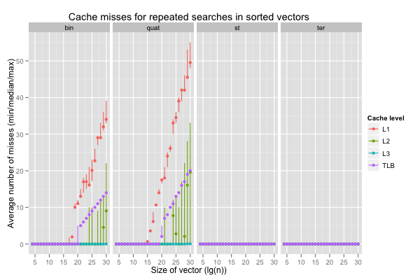
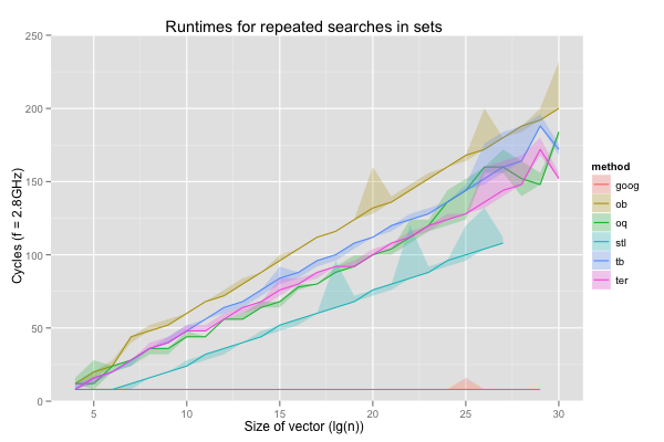
The next graph reports the performance of the methods when searching for the first element in sorted vectors, just to make sure we actually handle that case right. One would hope that the ternary searches (‘st’ for the serial loads, and ‘ter’ for the concurrent loads) improve on the binary (‘bin’) or quaternary (‘quat’) searches (that both suffer from aliasing issues); this is the reason we’re interested in them. We do observe a marked improvement in runtimes, and the second graph lets us believe it is indeed due to more successful caching (beware, the colours correspond to cache levels there, not search algorithms; there’s one facet for each search algorithm instead). Interestingly, \(\lg(n)=30\) is a bit faster than \(\lg(n)=29\) for the ternary searches; I can’t even hazard a guess as to what’s going on there.

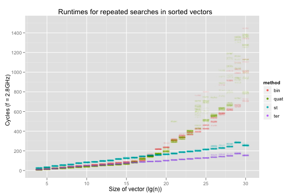
Additional MLP when the accesses cause many more cache misses doesn’t help. If anything, the performance of quaternary search is worse and less consistent than that of binary search. However, it does accelerate ternary search, for which caches work fine. The serial ternary search (‘st’) only improves on the binary or quaternary search for \(\lg(n)\geq 20\), where the classic search begin to really suffer from aliasing issues, but the ternary search with parallel loads (‘ter’) is always on par with the classic searches, or quicker.

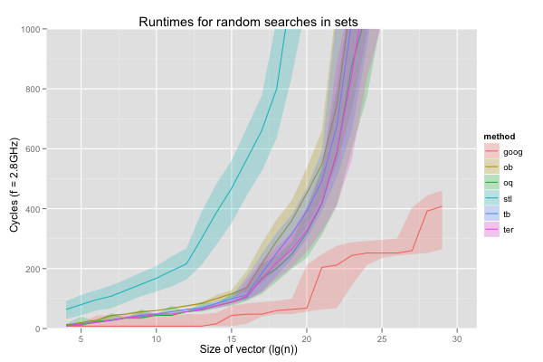
The next set of graph compares the performance of the methods when searching for random (present) keys; the same seed was used in each execution and for each method to minimise differences.

On this less easily cached workload, we find the same general effect on performance. Ternary search works better on larger vectors, and ternary search with parallel loads is faster even on small vectors, although the quaternary search seems to fare better here. Reassuringly, the ternary searches are also much more consistent, both in runtimes (narrower spreads in the runtime jittered plot), and in average cache misses, even with different physical memory allocation. The cache miss graph shows that, not surprisingly, the versions with parallel loads (quaternary and ternary searches) incur more misses than the comparable methods (binary and serial ternary), but that doesn’t prevent them from executing faster (see the runtime graph).

I draw two conclusions from these preliminary experiments: avoiding aliasing issues with slightly suboptimal subdivision (ternary searches) is a win, and so is exposing memory level parallelism, even when it results in more cache misses.

Enough with the preliminaries

The initial results let us exclude straight binary and quaternary search from consideration, as well as serial ternary search. We’re also know we’re looking for variants that avoid aliasing and expose memory-level parallelism.

Binary search is theoretically optimal (one bit of information to divide the range in two), so we could also try a very close approximation that avoids aliasing issues caused by exact division in halves. I implemented a binary search, with an offset-ed midpoint. Rather than guiding the recursion by the exact middle, the offset binary search reads from the \(31/63\)rd index (rounded up), and iterates on a subrange \(32/63\)rd as long. This is only slightly suboptimal: each lookup results in a division by \(63/32\), so that the off-center search goes through approximately 2.3% more lookups than a classic binary search. Comparing other methods with the offset binary search should be equivalent to comparing them with an hypothetical classic binary search free of aliasing issues.

Aliasing mostly happens at the beginning of the search, and ternary search is (theoretically) suboptimal. It may be faster to execute ternary search only at the beginning of the recursion (when aliasing stands in the way of caching frequently-used locations), and otherwise go for a classic binary search. I generated ternary/binary searches by using ternary search steps until the candidate range size was less than the square root of the original range size, and then switching to regular binary search steps.

Finally, quaternary search is interesting because it goes through roughly the same access patterns as binary search, but exposes more memory-level parallelism. Again, a very close approximation suffices to avoid aliasing issues; I went with reads at \(16/63\), \(32/63\) and \(1-16/63 = 47/63\), and iteration on a subrange \(16/63\)rd as long. Depending on the actual capacity for memory level parallelism during execution, it will perform between 51% and 152% as much work as binary search.

I also compared the performance of g++’s (4.7) STL set, and google’s dense_hash_set, which don’t search sorted vectors, but do work with sets, ordered or not.

The set in g++’s STL is a red-black tree with a fair amount of space overhead: each node has three pointers (parent, and left and right children) and a colour enum. For our data (32-bit unsigned), that’s about 700% additional space for each value. Even before considering malloc overhead, the set uses eight times as much memory as a sorted vector. Obviously, this affects the size of datasets that can fit in faster storage (data caches, TLB, or main memory)… on multi-socket machines, it also affects the size of datasets that can be processed before having to use memory assigned to a far-away socket. This is why the comparison for set was only performed until 128M 32-bit elements; after that, there wasn’t enough memory (a bit less than 12 GB) on the socket. In theory, the red-black tree is a bit less efficient than binary search, and probably in the same range as the ternary or quaternary searches: red-black trees trades potentially imperfect balancing (with some leaves at depth up to twice the optimum) for much quicker insertions. An interesting advantage of the red-black tree is that it naturally avoids aliasing issues: nodes will not tend to be laid out in memory following a depth-first, in-order traversal.

Google’s dense_hash_set is an open-addressed hash table with quadratic probing. It seems to target about 25% to 50% utilisation, so ends up using between four times or twice as much memory as the sorted vector. I’ve seen horrible implementations of tr1::hash for unsigned values in (it’s the identity function on my mac), so I wrote a quick tabular hash function. It’s very similar to the obvious implementation, but the matrix is transposed: when some octets are identical (e.g. all-zero high-order bits), the table lookups will hit close-by addresses. On the workloads considered here (small consecutive integers), the identity hash function would actually perform admirably well, but it would fail very hard on more realistic inputs. The tabular hash function is closer to the ideal, and makes the performance of the hash table nearly independent of the values constituting the set. It’s also pretty fast: we can expect the lookup table to fit in L2, and most probably in L1D, for the microbenchmarks used here.

1
2
3
4
5
6
7
8
9
10
11
12
13
14
15
16
17
18
19
20
21
22
23
24

struct hash_u32
{
        size_t tables[256][8];

        hash_u32()
        {
                for (unsigned i = 0; i < 256; i++) {
                        for (unsigned j = 0; j < 8; j++) {
                                size_t x = random(), y = random();
                                tables[i][j] = x^(y<<32);
                        }
                }
        }

        size_t operator() (unsigned x) const
        {
                unsigned x0 = x&0xff,
                        x1 = (x>>8)&0xff,
                        x2 = (x>>16)&0xff,
                        x3 = (x>>24)&0xff;
                return tables[x0][0] ^ tables[x1][1]
                        ^ tables[x2][2] ^ tables[x3][3];
        }
};

Comparing ordered sets with an unordered (hash) set may seem unfair: unordered sets expose fewer operations, and hash tables exploit that additional freedom to offer (usually) faster insertions and lookups. I don’t care. When I use a container, I don’t necessarily want an ordered or an unordered set. I wish to implement an algorithm, and that algorithm could well be adapted to exploit the strengths of either ordered or unordered sets. The dense hash table is a valid data point: it helps informs choices that happen in practice.

First, let’s compare these implementations – the hash table (‘goog’), the offset binary search (‘ob’), the offset quaternary search (‘oq’), the red-black tree (‘stl’), the ternary/binary search (‘tb’), and the ternary search (‘ter’) – on the two extreme cases we’ve been considering so far: constant searches for the least element, and searches for random elements. None of the algorithms suffer from aliasing issues, so the spread, if any, is smoothly covered. This allows me to avoid the rather busy jittered scatter plot and instead only interpolate between median cycle counts, with shaded regions corresponding to the values between the 10th and 90th percentile. The lines for ‘goog’ and ‘stl’ end early: these data structures could not represent the largest sets in the 12GB of local memory available in each processor. Also, now that we’ve dealt with the aliasing anomalies, I don’t feel it’s useful to graph the cache and TLB misses per size and implementation anymore.

When we always search for the least element in the set, the hash table obviously works very well: it only reads the same one or two cache lines, and they’re always in cache. Surprisingly, the red-black tree is also a bit faster than the searches in sorted vectors… until it exhausts all available memory. Looking at the behaviour on tiny sizes, it seems likely that the allocation sequence yields a nice layout for the first few steps of the search. The offset binary search is both faster and more consistent than the classic binary search (shown in earlier graphs), but never faster than the offset quaternary search. The ternary/binary search is similarly never faster than the straight ternary search.

On fully random searches, the hash table is obviously slower than when it keeps reading the same one or two words, but still much faster than any of the sorted sets. The red-black tree is now significantly slower than all the sorted vector searches (1000 cycles versus 200 to 400 cycles on vectors of 128K elements, for example). Again, we find that the offset quaternary search dominates the offset binary search, and the ternary search the hybrid ternary/binary search.

For the rest of the post, I’ll only consider google’s dense hash table, g++’s red-black tree, the offset quaternary search and the ternary search. Note that both the offset quaternary and ternary searches exhibit consistently better performance than the offset binary search, for which aliasing isn’t an issue. These alternative ways to search sorted vectors can thus be expected to improve on binary search even on vectors of lengths that are far from powers of two.

More interesting workloads

So far, I’ve only reported runtimes for two workloads: a trivial one, in which we always search for the same element, and a worst-case scenario, in which all the keys are chosen independently and randomly from all the values in the set (missing keys might be even worse for some hash tables). I see two dimensions along which it’s useful to interpolate between these workloads.

The first dimension is spatial locality. We sometimes work with very large sorted sets, but almost exclusively search for values in a small contiguous subrange. Within that subrange, however, there is no obvious relationship between search keys; we might as well be choosing them randomly, with uniform probability. The constant-element search is a degenerate case with a subrange of length one, and the fully random choice another degenerate case, with a subrange spanning the whole set. For all vector sizes from 1K to 1G elements, I ran the program with subranges beginning at the least value in the set and of size 1K, 16K, 64K, 256K, 1M and 2M (or size equal to the whole set if it’s too small). These values are interesting because they roughly correspond to working set sizes that bracket the cache and TLB sizes for all four implementations.

We can expect all methods to benefit from spatial locality, but not to the same extent. The hash table works well because it scatters everything pseudo-randomly in a large vector; when the subrange is sufficiently small compared to the set, each key in that subrange can be expected to use its own cache line, and the hash table’s performance will be the same as on randomly-chosen keys on relatively small subranges. Similarly, the red-black tree uses about eight times as much space as sorted vectors for the same data, and will also exceed the same cache level much more quickly.

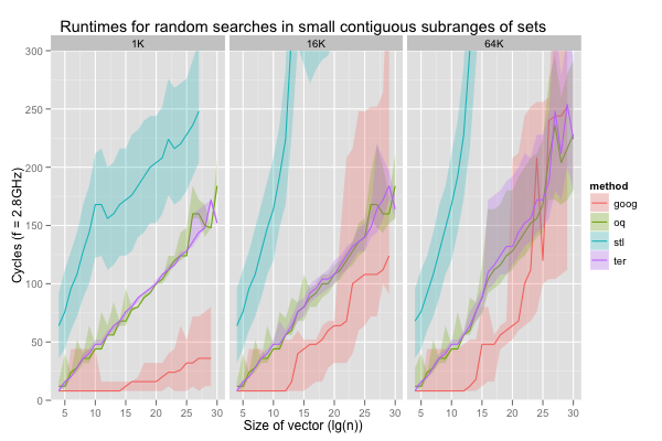
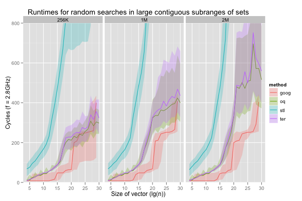
The red-black tree was slightly faster than the sorted vector searches when the key was always the same. This isn’t the case when the keys are selected from a small subrange. On all six scenarios and across all sizes, the 10th percentile for ‘stl’ is slower than the 90th for either ‘oq’ or ‘ter’. As expected, the runtimes for the hash table (‘goog’) evolve in plateaus, as the working set outstrips each level of caching. When it exceeds even the L3 (256K values in distinct cache lines is just barely larger than L3) its performance is more or less comparable to that of the sorted vector searches, as long as the subrange is below 2M items. All the sorted set implementations exhibit the same roughly sigmoidal shape for runtimes as functions of the set size. However, except for a few spikes on very large vectors, runtimes for the sorted vector searches grow much more slowly, and are more stable than for the red-black tree. In general, the offset quaternary search seems to execute a bit faster than the ternary search, but the difference is minimal. More importantly, when working with medium subranges (around 64K to 1M elements) in medium or large sets (1M elements or more), the sorted vectors searches are competitive with a hash table, in addition to being more compact.

The second dimension is temporal locality. I simulated workloads exhibiting temporal locality with strided accesses. For example with a stride of 17, the search keys are, in order, at rank 0, 17, 34, 51, etc. in the sorted set. The constant search is a special case with stride zero. For all vector sizes from 1K to 1G elements, I ran the programs with various strides: 1, 17, 65, 129, 257, and 1K+1. The ranks were taken modulo the set’s size, so these odd strides ensure that every key is generated for small vectors (i.e. they’re mod-1 step sizes, for corewar fans). The ordered sets should exploit this setting well (the red-black tree probably less so than the vector searches), and the hash table not at all: a good hash function guarantees that similar keys don’t hash to close-by values any more than very different keys, and the hash table will behave exactly as if keys were chosen randomly.

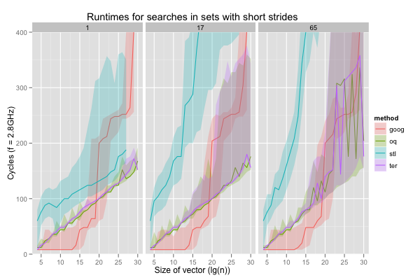
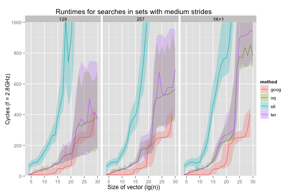
The hash table behaves almost exactly like it did with random keys; in particular, there is a large increase in runtimes when the set comprises at least 1M elements: the hash table then exceeds L3. Even on these very easy inputs, the red-black tree is only faster than the hash table on accesses with stride one, the very best case. Worse, the red-black tree already exhibits very wide variations (consider the height of the shaded areas for ‘stl’) on such traversals. It’s even wider on longer strides in large vectors, but the red-black tree is then also so slow that it’s completely off-graph. The sorted vector searches are always faster, and in general slightly more stable. In fact, they seem comparable with the hash table, if not faster, for nearly all vector sizes, as long as the access stride is around 129 or less.

From data to knowledge

I only worked on binary search here, and, even with this very simple algorithm, there are fairly obscure pitfalls. The issue with physical address allocation affecting cache line aliasing, particularly at the L2 level, is easy to miss, and can have a huge impact on results. Each execution of the test program showed very consistent timings, but different executions yielded timings that varied by a factor of two. We’ve been warned [pdf] about such hidden variables in the past, but that was a pretty stealthy instance with a serious effect.

Even without that hurdle, the slowdown caused by aliasing between cache lines when executing binary searches on vectors of (nearly-)power-of-two sizes is alarming. The ratio of runtimes between the classic binary search and the offset quaternary search is on the order of two to ten, depending on the test case. Some of that is due to MLP, but the offset binary search offers only slightly lesser improvements: aliasing really is an issue. And yet, I believe I haven’t seen anyone try to compensate for that when comparing fancier search methods that often work best on near-power-of-two sizes (e.g. breadth-first or van Emde Boas layouts) with simple binary search.

Also worrying is the fact that, even with all the repetitions and performance counters, some oddities (especially spikes in runtimes on very large vectors) are still left unexplained.

Nevertheless, these experiments can probably teach us something useful.

I don’t think that basing decisions on ill-understood phenomena is a good practice. This is why I try to minimise the number of variables and start with a logical hypothesis (in this case, “aliasing hurts and MLP helps”), rather than just being a slave to the p-value. Hopefully, this approach results in more robust conclusions, particularly in conjunction with quantile-based comparisons and a lot of visualisation. In the current case, the most useful conclusions seem to be:

1. use offset binary or quaternary search instead of binary search. Quaternary search is faster if the vectors are expected to be in cache, even when aliasing isn’t an issue, and both methods offer more robust performance;
2. good sorted sets can be faster than hash tables when reads tend to be strided, even with respectable strides on the order of 64 or 128 elements;
3. if the searches exhibit spatial locality over a couple hundred thousand bytes, searches in sorted vectors can be comparable to hash sets.

These raise two obvious questions: could we go further than quaternary search, and how do the results map to loopy implementations? I don’t think it’s useful to try and go farther than quaternary search: caches can only handle a few concurrent requests, and quaternary search’s three requests is probably close to, if not past, the maximum. In an implementation that’s not fully unrolled the offset searches are probably most easily adapted by multiplying the range by \(33/64 = 1/2+1/64\) or \(17/64 = 1/4+1/64\), with two shifts and a few adds. In either case, L2 cache misses tend to outweight branch mispredictions, which themselves are usually more important than micro-optimisations at the instruction level. The speed-ups brought about by eliminating aliasing and branches, while exposing memory-level parallelism, ought to be notable, even in a loopy implementation.